Package Walkthrough: TRU-OLS

Author

David Rach

Published

May 23, 2026

For the YouTube livestream schedule, see here

For screen-shot slides, click here

Background

There are different ways to unmix spectral flow cytometry data. TRU-OLS is one of them, with the methodology behind the approach explained in this 2025 Cyto Part A paper by Ryan Kmet and David Novo.

Logistics

It is implemented in the Julia programming language. Since this is a Cytometry in R course (and I have no plans to implement a Cytometry in Julia course), we will need to figure out a few logistics first. Namely…

We will need to retrieve the information we need for unmixing from the raw .fcs files in R
Hand off these intermediate outputs to Julia (either directly or via the JuliaCall R package)
After unmixing has been carried out, return these outputs to R, and integrate them back into a properly formatted .fcs file

In this walk-through, we will see a basic example of how this can be implemented, leveraging what we know about the R programming language, plus select targeted google searches, to allow us to pass what is needed to Julia, and then get the returned objects back into R.

If we manage to get these three goals accomplished, we will be able to unmix our data using TRU-OLS, and end up will properly set up .fcs files that can be opened with any flow cytometry software.

Method

Note

The following notes about TRU-OLS arose as part of a Cytometry Discord discussion thread within the “data” channel on August 25, 2025 discussing the released paper. As a community “Journal Club”, some important details may have been missed. All screenshots (and badly hand-scrawled notes) originate from the paper figures. The thread is reposted below with minimal editing.

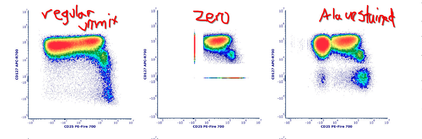
Background: As we increase number of markers in the unmixing matrix, variance contributes to increasing amounts of noise around the negative population. This was illustrated recently in the Mair and Mage paper. For the unstained sample iteratively unmixed up to 40 markers, you can see how this spreads out. 1/n

The way TRU-OLS seems to work relies on the unmixing controls (single color and unstained). Single colors are used to provide the signatures for the full matrix. The unstained is then unmixed against this matrix. A cutoff point is then set at the 99.5% (very right edge) of the spread. This cutoff is used to help determine for individual cells what fluorophores are present before downsizing the matrix to only the relevant fluorophores. 2/n

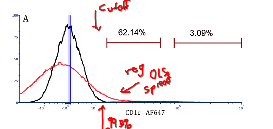
Consequently, for the full-stained sample, each cell is initially unmixed. If the value is below the cutoff set by the unstained spread, the marker is presumed negative and removed from the re-unmix matrix. Once all the “irrelevant” fluors are removed, the full-stained cell is reunmixed with the remaining fluorophore matrix. 3/n

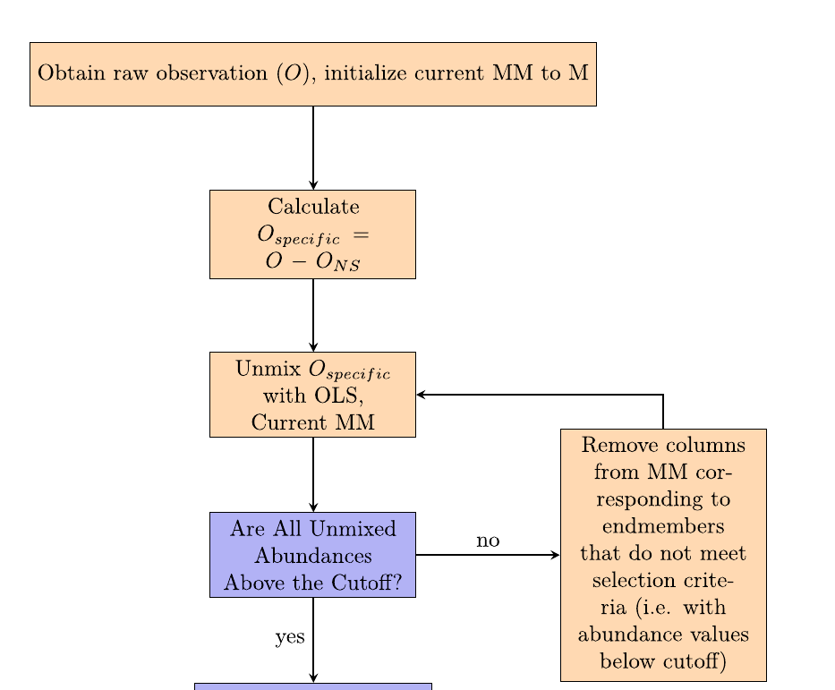
Finally, the “irrelevant” fluorophores on the re-unmixed cell can be either set to 0, or reorganized into the original spread of the unstained negative. 4/n

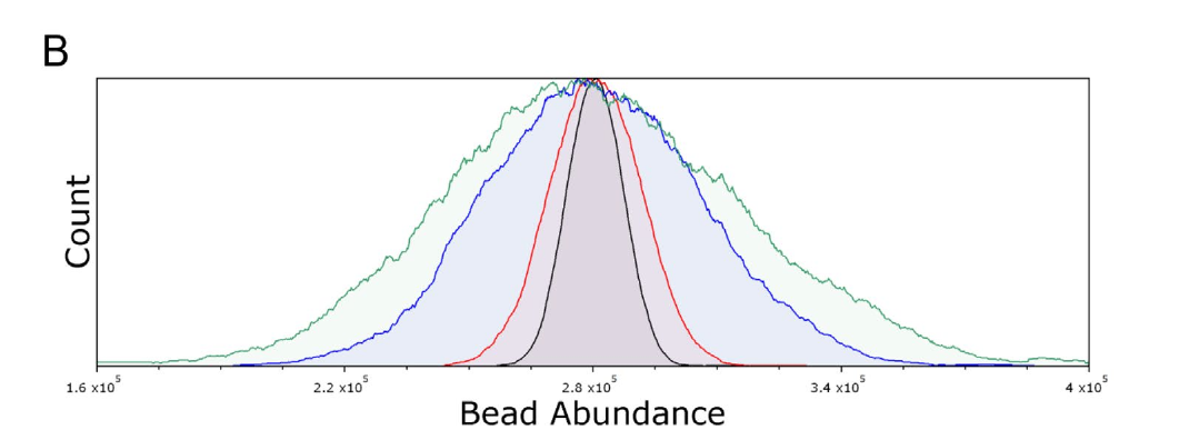
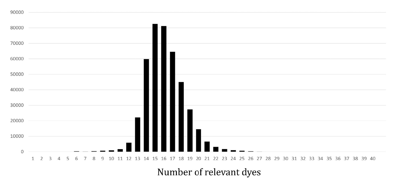
When enumerating how many markers were retained for the individual re-unmixing, we see following distribution of “smaller matrices used”. 5/n:

In addition to removing all events below the cutoffs, the removal of “irrelevant” markers results in the Bermuda zone between the cutoff and the bright population to also clean up when comparing between regular OLS unmixing and the TRU-OLS approach. 6/n.

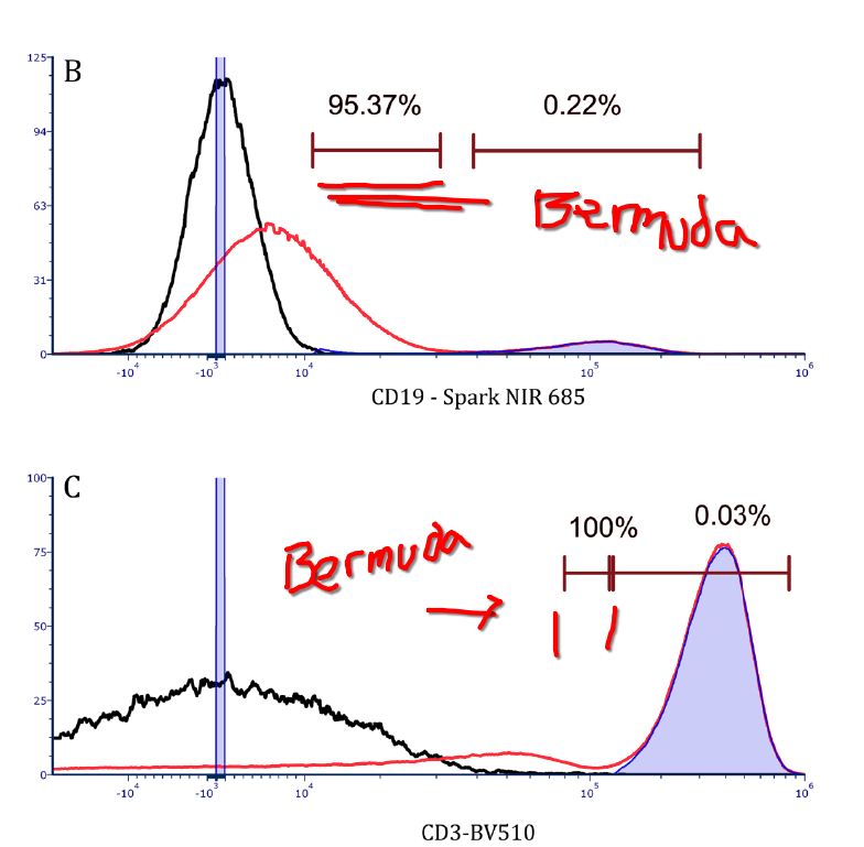
The approach makes the most difference on cells where there wasn’t much marker co-expression to begin with. For the heavily co-expressed cells, everything is kept, and their uncertainty still persist as spread. 7/n.

My outstanding questions is one, if we are depending on the positive peaks remaining in the same place based on the reference, how does this work for cells across multiple individuals in practice. Likewise, I will need to play around with more dim population data before I can vouch haven’t also thrown the baby out with bathwater. With that said, I like it.

Walk-through

Setup

Before getting started, let’s make sure that both the Julia programming language is installed on our local computer, and then proceed to download TRU-OLS and make sure it is active in our local environment.

Installing Julia

Since how you install Julia will vary depending on your computer operating system, please see these instructions. Once Julia has been successfully installed, please return and proceed to the next step.

Downloading TRU-OLS

As of the moment, TRU-OLS is available via GitHub. Consequently, we are able to download it similar to any GitHub-based code to make it available on our local computer. To simplify the installation process (and allow us to make any necessary changes should we encounter dependency version issues later on), I recommend going ahead and forking the repository. This additionally helps the authors track usage and community interest in their work.

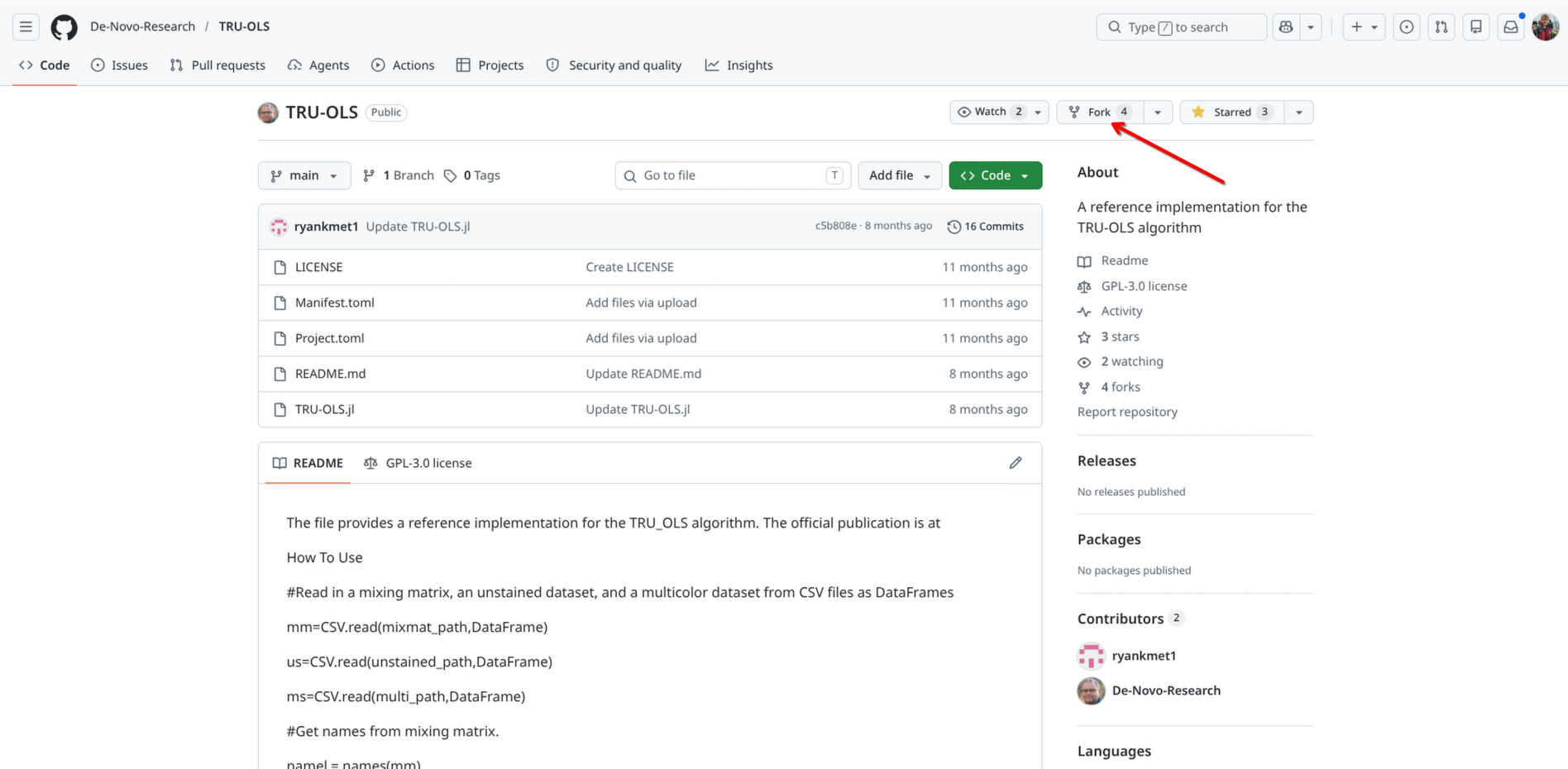
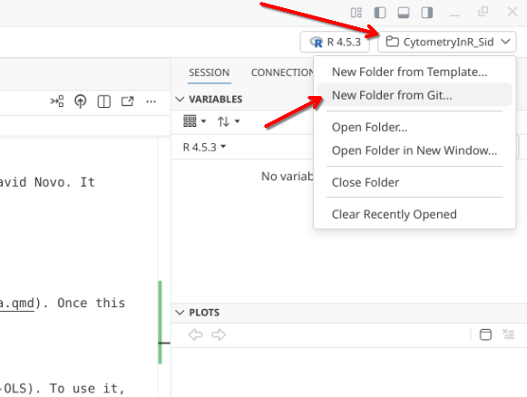
After forking the project to your own GitHub account, copy the url, open up Positron, and select the drop-down option on the upper-right to create a New Folder from Git.

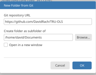
Paste in the url to your forked version of TRU-OLS, and proceed with the download.

Following completion, open the new project folder inside Positron.

Activating TRU-OLS

To begin using TRU-OLS, just like any R package, we are going to need to make sure the required dependencies are installed. These are documented inside the “Manifest.toml” file. To get started, proceed to your terminal tab and run the following line of Julia code

# Julia code
julia --project=.

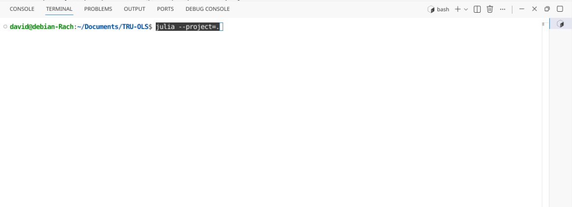
The Julia splash screen will then be displayed within the terminal window

Now that Julia is active in our terminal, we will see julia> appearing on each line. Proceed to type (or paste) the following code to commence the installation of the required dependencies.

# Julia code
using Pkg
Pkg.instantiate()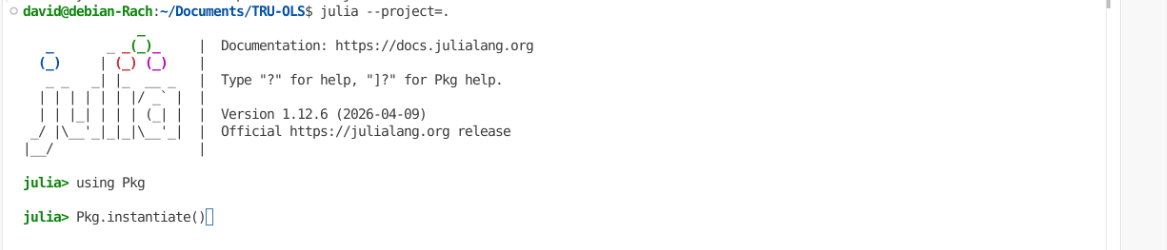

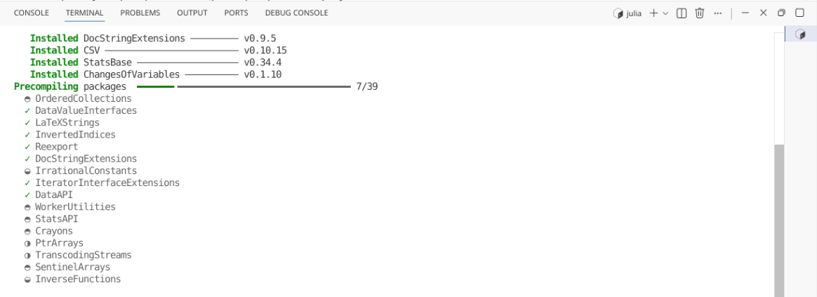
The installation of the required Julia packages will then proceed, with the status of the various steps (including installation and pre-compiling) being displayed

In my attempt to install the dependencies, I ended up with an error when installing the CSV package.

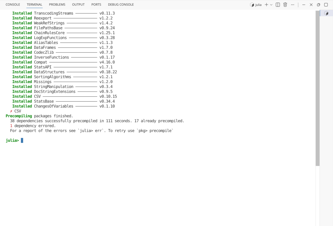
# Julia code
err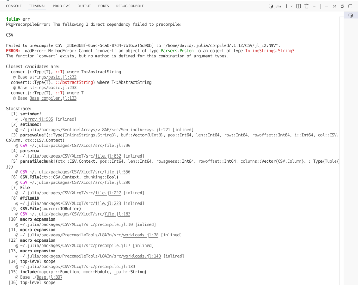

Similar to when we encounter errors installing an R package, we can apply those same troubleshooting skills in this context. First glancing at the “Manifest.toml” file, the original manifest list the Julia version 1.8.5. In my case, my installed Julia version was more recent (1.12.6), suggesting we likely have a dependency clash due to the older version listed in the manifest.

I decided to re-run Pkg.instantiate(), and as we would anticipate, I still retrieved the previous error

# Julia code
using Pkg
Pkg.instantiate()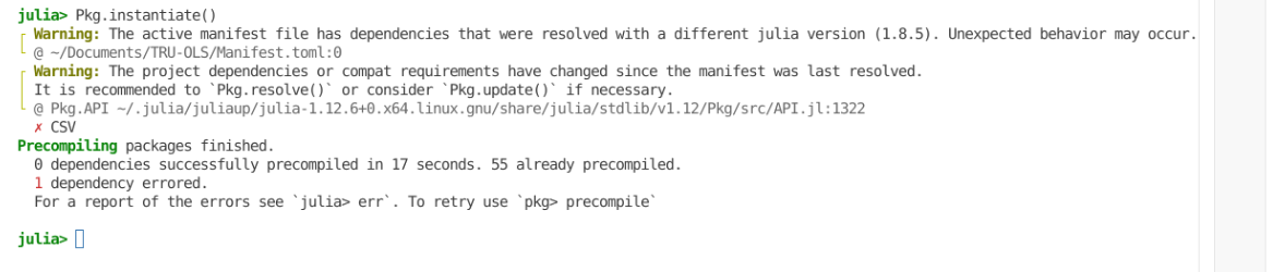

However, in this case, the message output suggested the use of Pkg.resolve(), which I next attempted

# Julia code
using Pkg
Pkg.resolve()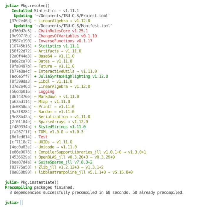

Based on the Positron highlighting syntax, this resulted in a few package additions and deletions. On re-running Pkg.instantiate(), the CSV package successfully installed.

Checking the Source control tab in the actions bar, and clicking on the “Manifest.toml” file, we can see the different updates that were effectuated by Pkg.resolve()

Once this was done, I saved my changes to the files, staged them to version control, wrote a short commit message, before pushing everything from my local fork back to GitHub. This prevents the need to repeat the troubleshooting process next time I needed to set TRU-OLS up on another computer in the future.

Dataset

For this walkthrough, the spectral flow cytometry .fcs files being used were generated in 2025 as part of the yearly 5-day training workshop here at UMGCCC FCSR. The panel consisted of 5 markers (CD45, CD3, CD4, CD8 and Viability). This panel was used to stain mouse splenocytes, which were then acquired on a 5-laser Cytek Aurora.

Loading FCS files to GatingSet

With both Julia and TRU-OLS now installed, switch back to the R project folder that you will be primarily be working in for unmixing.Once there, you will need to load your unmixing controls and full-stained samples into a GatingSet.

As always, start by attaching to your local environment the required R packages via the library() call

library(flowWorkspace)

As part of improvements to flowWorkspace, some behavior of
GatingSet objects has changed. For details, please read the section
titled "The cytoframe and cytoset classes" in the package vignette:

  vignette("flowWorkspace-Introduction", "flowWorkspace")

library(flowGate)

Loading required package: ggcyto

Loading required package: ggplot2

Loading required package: flowCore

Loading required package: ncdfFlow

Loading required package: BH

library(dplyr)


Attaching package: 'dplyr'

The following object is masked from 'package:ncdfFlow':

    filter

The following object is masked from 'package:flowCore':

    filter

The following objects are masked from 'package:stats':

    filter, lag

The following objects are masked from 'package:base':

    intersect, setdiff, setequal, union

library(purrr)
library(JuliaCall)

Next off, specify the storage location of the .fcs files, and also the location of the folder you want any unmixed fcs files to be saved to.

#StorageLocation <- file.path("course", "community", "TRU-OLS", "data")
StorageLocation <- file.path("data")

#OutputLocation <- file.path("course", "community", "TRU-OLS", "outputs")
OutputLocation <- file.path("outputs")

Proceed to load the identified .fcs files into a GatingSet object

fcs_files <- list.files(StorageLocation, pattern=".fcs",
 full.names=TRUE, recursive=TRUE)

SFC_cytoset <- load_cytoset_from_fcs(fcs_files,
 truncate_max_range=FALSE, transformation=FALSE)
SFC_GatingSet <- GatingSet(SFC_cytoset)

As we will be working with raw .fcs files for the unmxing process, we do not need to transform, as we need signatures retrieved from the underlying data to appear in their normal shapes.

I recommend then using subset() on the GatingSet, placing the single-color and unmixing controls into their own GatingSets, and repeating the process for the full-stained samples. This ensures we only retrieve signatures from the single-color controls, and that only the full-stained samples are unmixed.

# pData(SFC_GatingSet)

FullStain_GS <- subset(SFC_GatingSet, name == "Full-Stained2_scatter.fcs")

Unstained_GS <- subset(SFC_GatingSet, name == "Unstained (Cells)_scatter.fcs")

UnmixingControl_GS <- subset(SFC_GatingSet, name != "Full-Stained2_scatter.fcs" &
   name != "Unstained (Cells)_scatter.fcs")

Signature Matrix

To facilitate this example, we will use the Luciernaga_SingleColors() function from the Luciernaga package to retrieve the signatures from our single-color controls. For more information, please see the vignette.

# remotes::install_github("DavidRach/Luciernaga")
library(Luciernaga)

# Define the primary detectors

UnmixingPanel <- data.frame(
  Fluorophore = c("BV510-A", "BV605-A", "Spark Blue 550-A", "7-AAD-A", "Alexa Fluor 700-A"),
  Detector = c("V7-A", "V10-A", "B3-A", "YG4-A", "R4-A"))

# Define what brightness percentiles to include

ThePanelCuts <- UnmixingPanel |> select(-Detector) |> mutate(From=0.8) |> mutate(To=1)

# Extract the signatures 

SCs <- map(.x=UnmixingControl_GS, .f=Luciernaga_SingleColors, sample.name="TUBENAME",
 removestrings=c(".fcs", "PD_AD_"), subset="root", PanelCuts=ThePanelCuts, stats="median", Verbose=FALSE, 
 SignatureView=TRUE) |> bind_rows()

SCs

      Fluorophore    Ligand     UV1-A     UV2-A    UV3-A    UV4-A     UV5-A
1  Spark Blue 550       CD3 104.74154 188.68995 420.2939 594.9452  864.0328
2           BV605       CD4  79.07824 158.78110 496.5042 651.8056  871.7632
3 Alexa Fluor 700      CD45 107.72574 219.83228 498.7449 701.1989 1017.6757
4           BV510       CD8 121.22008 231.06911 546.3041 832.8344 1744.4631
5           7-AAD Viability  75.56364  73.38842  87.1750  86.8321  131.5948
      UV6-A      UV7-A      UV8-A     UV9-A     UV10-A    UV11-A    UV12-A
1 1495.2246  2580.6736  2742.1285  2186.741   688.7473  312.4049  191.5149
2 1413.0586  2221.1409  1417.7964  7160.168 13850.0234 6889.8103 2858.5405
3 1794.0203  2884.1611  1783.2721  1394.581   432.0355  269.5648  965.4911
4 5374.4111 25075.5771 21001.8184 17206.926  6222.8848 2291.9504 1099.8838
5  224.5899   322.6273   235.3316   536.639  1366.8877 3236.7268 2164.1993
     UV13-A    UV14-A    UV15-A    UV16-A       V1-A      V2-A      V3-A
1  140.9085  153.3083  146.2526  135.8367  142.32812  364.2118  472.9013
2 2163.7251 1983.9139 1231.0778  862.3104 4854.59058 6594.5967 5717.8762
3 4073.7609 4180.7432 2346.9130 1820.5828  147.33545  392.1243  528.0650
4  762.3667  746.6266  530.1944  411.1842  229.92508 1765.3419 6732.9707
5 1850.2953 1949.2087 1384.9995 1028.7186   56.95234  187.5039  268.9663
        V4-A       V5-A       V6-A       V7-A       V8-A       V9-A      V10-A
1   467.2418   891.2451  3398.5063 10576.7729  6412.2529  4036.4619  3800.3064
2  3200.3501  1989.8629  1320.9020  1545.9777 14717.8267 56108.5410 69693.8047
3   522.9897   805.8846   800.3869  1068.3057   784.9185   531.3835   594.9357
4 14236.3481 37583.2031 39042.7402 53597.5996 37457.4648 23858.7520 24001.5322
5   281.9515   383.5099   349.8906   424.0339   979.9825  2716.0559 11870.2383
       V11-A      V12-A      V13-A      V14-A     V15-A     V16-A      B1-A
1  1398.0156   729.8098   610.9025   482.7387  406.1053  211.9564 1727.9603
2 33012.0508 13375.8213 10442.9980  6913.8130 4227.4131 1816.5377  472.0234
3   410.3605  3569.9545 18858.6064 13525.6689 7742.5754 3852.9854  485.0185
4  8262.2681  3854.7830  2837.6615  1933.1819 1358.4150  576.0975  587.8901
5 19976.5449 13250.9321 11821.9834  9180.0054 6730.8584 3196.4229  147.2456
        B2-A       B3-A       B4-A      B5-A       B6-A       B7-A       B8-A
1 11803.6841 31791.0898 13055.8618 9729.2339  5960.7681  3127.5720  2222.0243
2   442.6214   540.6498   738.8925 2996.0658  2870.6008  2005.9507  1302.9653
3   469.6182   560.3932   305.5835  339.6832   244.6713   152.8191   210.2808
4   554.4593   658.5273   372.5866  380.8456   288.1743   165.7359   140.0763
5   155.3411   214.6584  1326.2528 5897.7673 20978.9561 54340.7949 46198.2520
        B9-A      B10-A       B11-A      B12-A       B13-A       B14-A
1  2092.9392  1235.8806   801.18732   685.7439   506.45784   602.38147
2  1045.8303   616.8634   411.57971   301.7630   210.75192   234.18474
3  1098.3724  2552.8210  1888.99933  1150.0874   777.24994   927.87350
4   146.0795   108.9569    69.67178    74.3706    55.30247    71.59775
5 49241.4121 30504.1377 19612.47266 17056.9932 12517.82764 13991.46777
      YG1-A       YG2-A       YG3-A       YG4-A        YG5-A       YG6-A
1  728.4496   412.28871   294.84369    225.3277    122.32074   123.49529
2 4960.2808 23393.29395 23929.44727  15121.0571   9115.67529  6222.96021
3  173.3573    88.36777   109.43902    267.5920    776.15417  5119.80396
4  193.2470    99.99137    92.44199    164.6935     92.89421    81.73549
5 3614.0844 13031.28711 40427.65039 124554.5195 101246.96484 93211.57812
        YG7-A       YG8-A       YG9-A      YG10-A       R1-A       R2-A
1    159.5041    86.86105    60.32009    49.90587   59.36887   65.15396
2   6832.3105  2701.12439  1620.54364   951.89786  127.81407  119.96352
3  29223.2451 12844.04395  7387.60693  4942.44336  370.45784 4182.69580
4    126.0765    67.43141    54.69088    66.03951   69.02694   71.98460
5 112102.7891 51718.50781 38361.86328 23770.70703 1828.64563 2459.72717
         R3-A         R4-A        R5-A        R6-A        R7-A        R8-A
1    58.51100     53.43020    36.55869    50.95368    65.37681    22.83324
2   107.51331     96.55773    79.32631    83.67997    79.76941    45.79163
3 37749.57227 103404.82812 94201.42188 46773.15820 44290.40430 25535.98047
4    76.35984     66.68982    53.12717    64.87876    73.56101    36.30670
5  2500.10327   1926.56720  1511.25427  1097.58972  1131.22571   595.57352

Let’s also visualize the signatures against the reference signatures for the respective fluorophores to ensure that the retrieved signatures are appropiate.

plots <- map(.x=UnmixingControl_GS, .f=Luciernaga_SingleColors, sample.name="TUBENAME",
 removestrings=c(".fcs", "PD_AD_"), subset="root", PanelCuts=ThePanelCuts, stats="median", Verbose=FALSE, SignatureView=TRUE, returntype="plots")

plots

[[1]]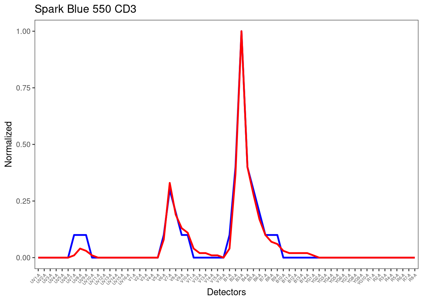


[[2]]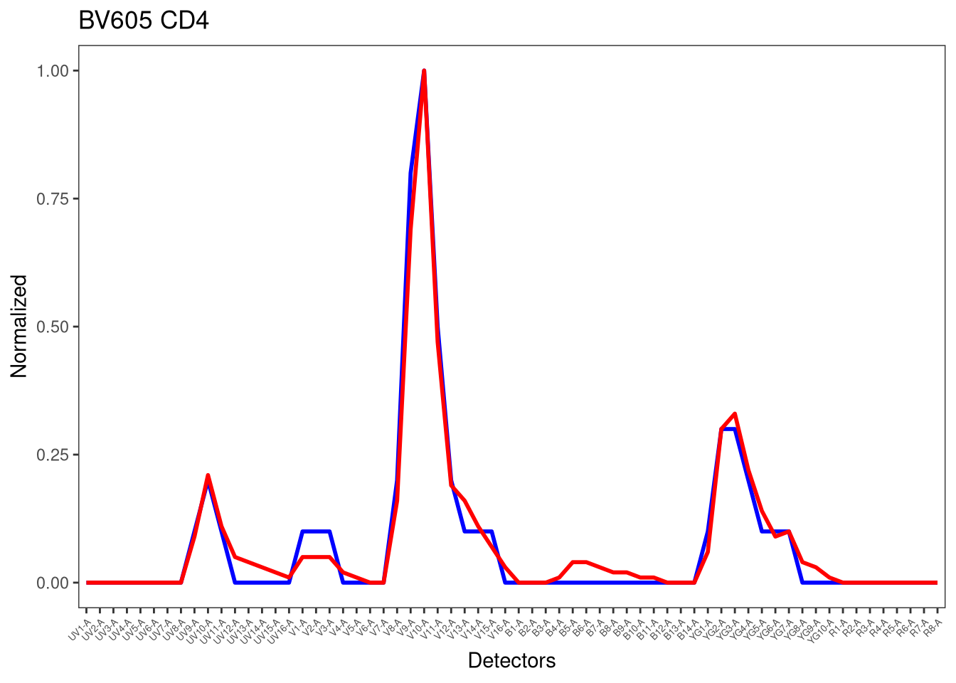


[[3]]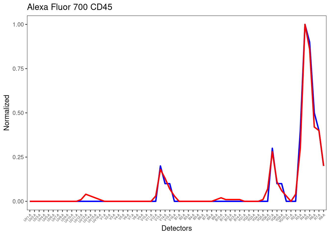


[[4]]


[[5]]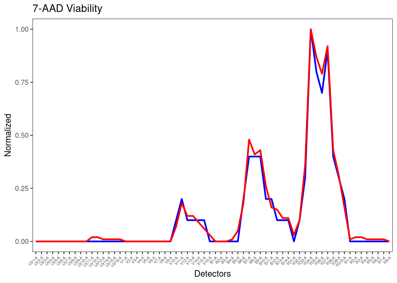

In this case, the signatures are close enough to the reference that we can proceed (the rough edges are likely result of the datasets single-color unmixing controls being severely downsampled in order to pass the GitHub size limits)

OLS-Unmixing via Luciernaga

Since we may be interested in comparing how TRU-OLS unmixing differs compared to regular OLS unmixing (and since we have already generated the needed inputs), lets proceed to unmix via Luciernaga and generate an .fcs file to our designated outputs folder for later.

TheSampleName <- c("TUBENAME")

UnmixSuccess <- map(.x=FullStain_GS, .f=Luciernaga_Unmix,
 controlData=SCs, sample.name=TheSampleName, addon="_Luciernaga_Unmixed", subset="root", removestrings="fcs", outpath=OutputLocation, PanelPath=UnmixingPanel, Verbose=TRUE)

After removestrings, name is Full-Stained2

TRU-OLS Unmixing

Within the TRU-OLS README, we are given a few line of codes with instructions on how to run

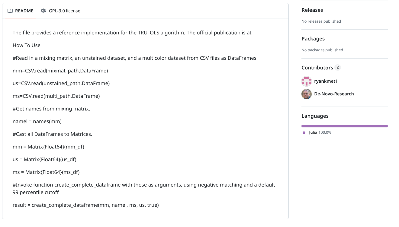
The main inputs are three csv files that are read into JUlia, mixmat (the signature matrix of the single-colors), unstained (the cleaned up exprs output for the unstained sample), and multi (the cleaned up exprs outputs for the full-stained sample). The names of the fluorophores are then subsequently retrieved from the mixmat file.

These data.frames are then all converted to matrices, before being passed off to create_complete_dataframe() function, which runs using the default parameters.

From previous function building examples, we have enough familiarity with the flowWorkspace package to figure out how to retrieve and clean up the exprs() output in R to fulfill the inputs needed for unstained and full-stained samples to be passed to Julia. We can also use Luciernaga_SingleColors() to generate the mixmat data.frame of fluorophore signatures.

After attempting (and failing) to pass from an R code chunk to a Julia code chunk, I found the implementable approach was to write the data.frames to .csv files, and then via JuliaCall package run Julia commands within the R function to carry out the above README suggested steps, and save the output as a .csv file that could be read back into R.

The main thing needed was to provide the correct file path to the TRU-OLS.jl file with the corresponding Julia code.

#' Implements TRU-OLS unmixing in Julia, via the JuliaCall R package. 
#' 
#' @param mixmat The signature matrix
#' @param unstained The cleaned up exprs of the unstained
#' @param fullstained The cleaned up exprs of the full-stained
#' @param TRUOLSPATH File.path to the TRU-OLS.jl file
#' 
#' @importFrom JuliaCall julia_setup julia_command 
#' @importFrom utils read.csv write.csv
#' 
TRU_OLS_Julia <- function(mixmat, unstained, fullstained,
 TRUOLSPath="/home/david/Documents/TRU-OLS/TRU-OLS.jl") {

  library(JuliaCall)
  write.csv(mixmat,      "mixmat.csv",      row.names=FALSE)
  write.csv(unstained,   "Unstained.csv",   row.names=FALSE)
  write.csv(fullstained, "FullStained.csv", row.names=FALSE)
  
  julia_setup()
  julia_command('import Pkg; Pkg.add(["CSV", "DataFrames", "LinearAlgebra", "StatsBase", "FileIO", "FCSFiles"])')
  julia_command('using CSV, DataFrames')
  julia_command('mm = CSV.read("mixmat.csv", DataFrame)')
  julia_command('us = CSV.read("Unstained.csv", DataFrame)')
  julia_command('ms = CSV.read("FullStained.csv", DataFrame)')
  julia_command('namel = names(mm)')
  julia_command('mm = Matrix{Float64}(mm)')
  julia_command('us = Matrix{Float64}(us)')
  julia_command('ms = Matrix{Float64}(ms)')
  julia_command(sprintf('include("%s")', TRUOLSPath))
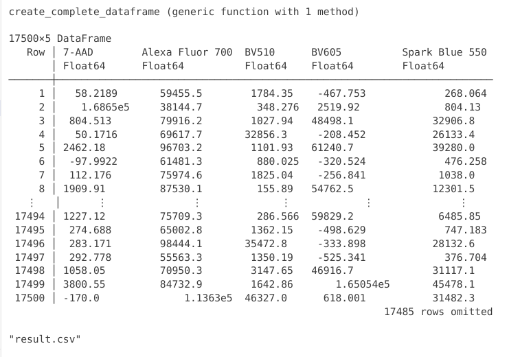
  julia_command('result = create_complete_dataframe(mm, namel, ms, us, true)')
  julia_command('CSV.write("result.csv", result)')
  
  result_r <- read.csv("result.csv", check.names=FALSE)
  return(result_r)
}

With the “R to Julia and back to R” hand-off operational, the main thing left is to provide the function infrastructure in R needed to gather the required inputs, and then once the outputs are received, correctly package them back into a new .fcs file. I modified the existing function infrastructure for Luciernaga_Unmix() used for the OLS unmixing example above, but switching out the OLS unmixing with the TRU_OLS_Julia() function we just wrote.

#' @param x An interated-in full-stained raw .fcs file needing to be unmixed
#' @param SCs The fluorophore signature matrix generated via Luciernaga_SingleColors
#' @param Unstained_GS The GatingSet containing the raw unstained fcs file
#' @param sample.name The keyword containing the fcs file name
#' @param removestrings A list of values to remove from name
#' @param Verbose For troubleshooting name after removestrings
#' @param addon Additional addon to append to the new .fcs file name
#' @param subset A gating hierarchy level to sort cells at, expression values retrieved
#' from these
#' @param outpath The return folder for the .fcs files
#' @param PanelPath Location to a panel.csv containing correct order of fluorophores
#' @param returnType Whether to return "fcs" or "flowframe"
#' @param TRUOLSPATH File.path to the TRU-OLS.jl file
#' 
#' @importFrom JuliaCall julia_setup julia_command 
#' 
TRUOLS_Unmix <- function(x, SCs, Unstained_GS, sample.name, removestrings,
   Verbose, addon, subset="root", outpath, PanelPath, returnType="fcs",
   TRUOLSPath = "/home/david/Documents/TRU-OLS/TRU-OLS.jl"){

  # File Name Clean Up

  if (length(sample.name) == 2){
      first <- sample.name[[1]]
      second <- sample.name[[2]]
      first <- keyword(x, first)
      second <- keyword(x, second)
      name <- paste(first, second, sep="_")
    } else {name <- keyword(x, sample.name)}

    name <- NameCleanUp(name, removestrings=removestrings)
    if (Verbose == TRUE){message("After removestrings, name is ", name)}

  # Normalize the Single Color Signature Matrix (important for final scaling)

  if (any(SCs |> select(where(is.numeric)) > 1)){
    Metadata <- SCs |> select(!where(is.numeric))
    Numerics <- SCs |> select(where(is.numeric))
    n <- Numerics
    n[n < 0] <- 0
    A <- do.call(pmax, n)
    Normalized <- n/A
    SCs <- bind_cols(Metadata, Normalized)
 }

    # Formating SingleColors to required mixmat format
    SCsM <- t(SCs)
    mixmatDF <- data.frame(SCsM)
    colnames(mixmatDF) <- mixmatDF[1,]
    Ligands <- mixmatDF[2,] |> unlist() |> unname()
    mixmatDF <- mixmatDF[3:nrow(mixmatDF),]
    mixmat_mat <- as.matrix(mixmatDF)

    # Extracting the Unstained Detectors exprs values
    Unstained <- gs_pop_get_data(Unstained_GS, "root")
    Unstained <- flowCore::exprs(Unstained[[1]])
    UnstainedDF <- data.frame(Unstained, check.names=FALSE)
    UnstainedDF <- UnstainedDF[!stringr::str_detect(names(UnstainedDF), "FSC|SSC|Time")]
    Unstained_mat <- as.matrix(UnstainedDF)

    # Extracting the Full-Stained Detectors exprs values
    FullStainedCS <- gs_pop_get_data(x, "root")
    FullStained <- flowCore::exprs(FullStainedCS[[1]])
    FullStainedDF <- data.frame(FullStained, check.names=FALSE)
    StashedDF <- FullStainedDF[stringr::str_detect(names(FullStainedDF), "FSC|SSC|Time")]
    FullStainedDF <- FullStainedDF[!stringr::str_detect(names(FullStainedDF), "FSC|SSC|Time")]
    FullStained_mat <- as.matrix(FullStainedDF)

    # Unmixing via the R-Julia wrapper function
    TheUnmixed <- TRU_OLS_Julia(mixmat=mixmat_mat, unstained=Unstained_mat,
    fullstained=FullStained_mat, TRUOLSPath = TRUOLSPath)

    # Returning Time, FSC, SSC columns back in to the unmixed file
    TheOrder <- SCs |> pull(Fluorophore)
    TheLigands <- SCs |> pull(Ligand)
    TheUnmixed <- TheUnmixed[, TheOrder]
    TheData <- cbind(StashedDF, TheUnmixed)
    rownames(TheData) <- NULL
    StandInStashed <- StashedDF |> mutate(Backups=row_number()) |> relocate(Backups, .before=1)

    # Handoff to Luciernaga Internal Unmix for the .fcs formatting
    new_fcs <- Luciernaga:::InternalUnmix(cs=FullStainedCS,
    StashedDF=StandInStashed, TheData=TheData, Ligands=TheLigands)

    # Modifying the filename
    if (!is.null(addon)){name <- paste0(name, addon)}
    AssembledName <- paste0(name, ".fcs")
    new_fcs@description$GUID <- AssembledName
    new_fcs@description$`$FIL` <- AssembledName

    # Sending the file out as an .fcs file
    if (is.null(outpath)) {outpath <- getwd()}
    fileSpot <- file.path(outpath, AssembledName)
    if (returnType == "fcs") {write.FCS(new_fcs, filename = fileSpot, delimiter="#")
    } else {return(new_fcs)}
}

With both the main function (and the internal R-Julia handoff function) written and active in our environment, we can now proceed to unmixing.

UnmixSuccess <- map(.x=FullStain_GS, .f=TRUOLS_Unmix, SCs=SCs, Unstained_GS=Unstained_GS, 
 sample.name=TheSampleName, addon="_TRUOLS_Unmixed", subset="root",
 removestrings="fcs", outpath=OutputLocation, PanelPath=UnmixingPanel, Verbose=TRUE)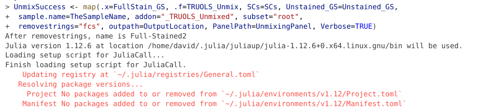

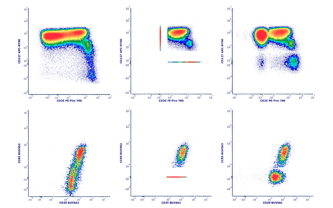
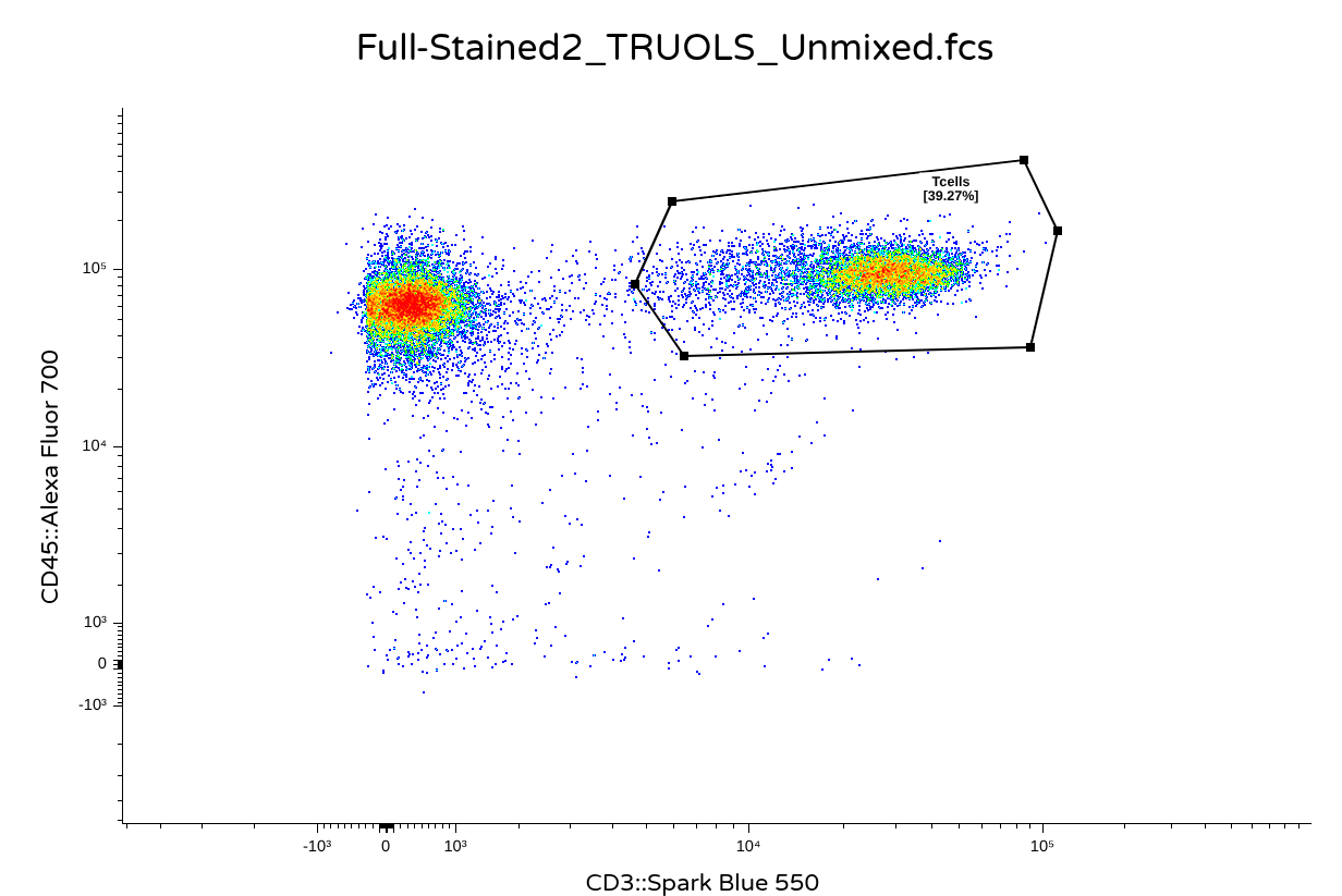
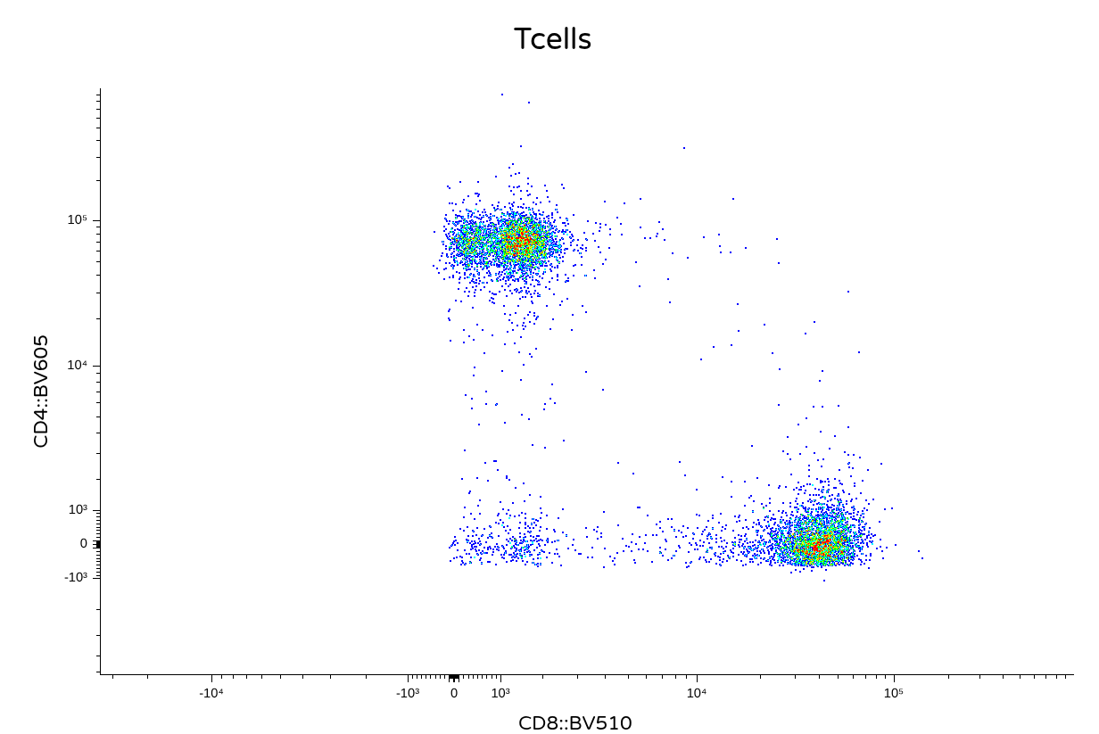
And for a quick sanity check, lets check both the OLS and TRU-OLS files to make sure that the .fcs file formatting worked in practice.

OLS

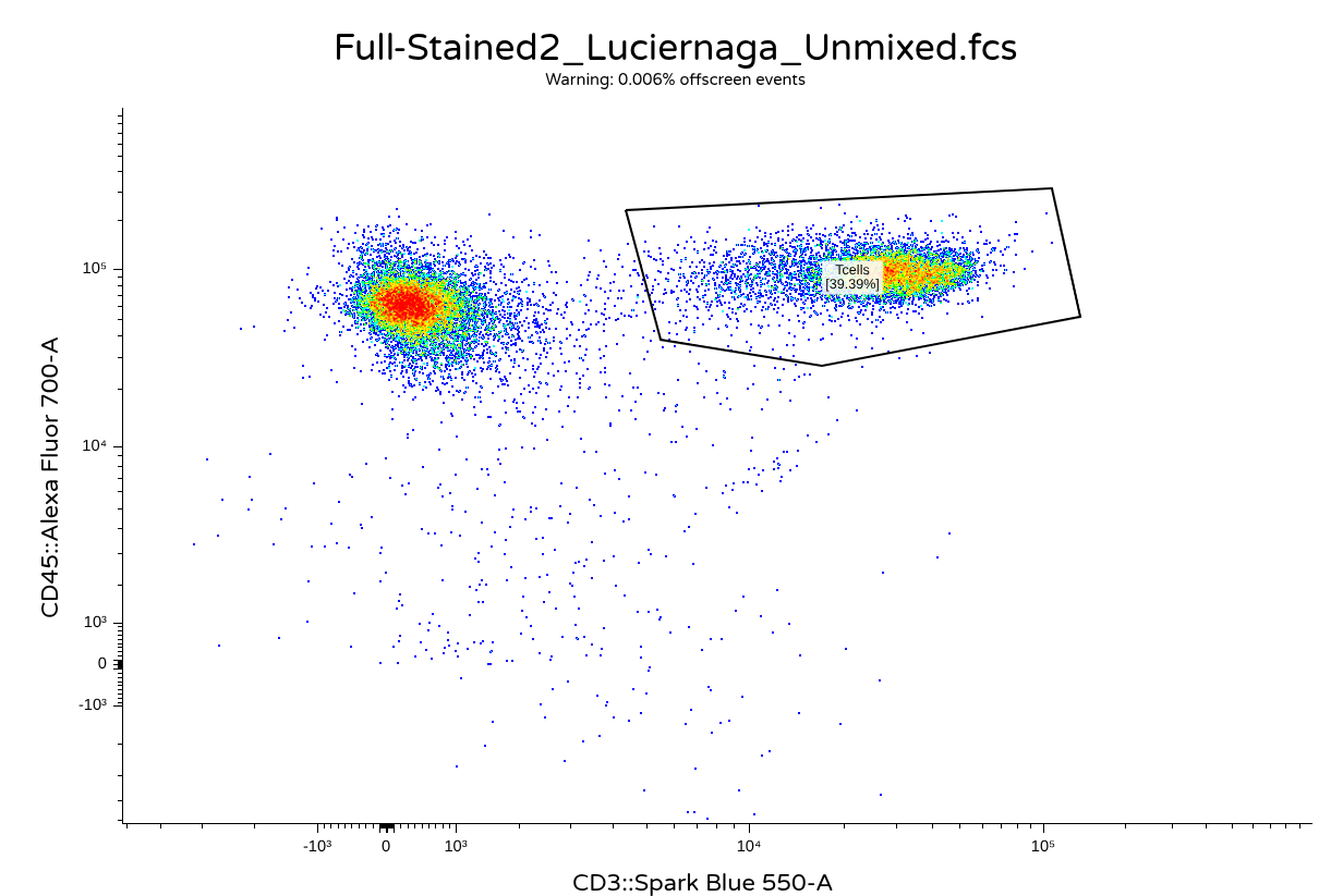
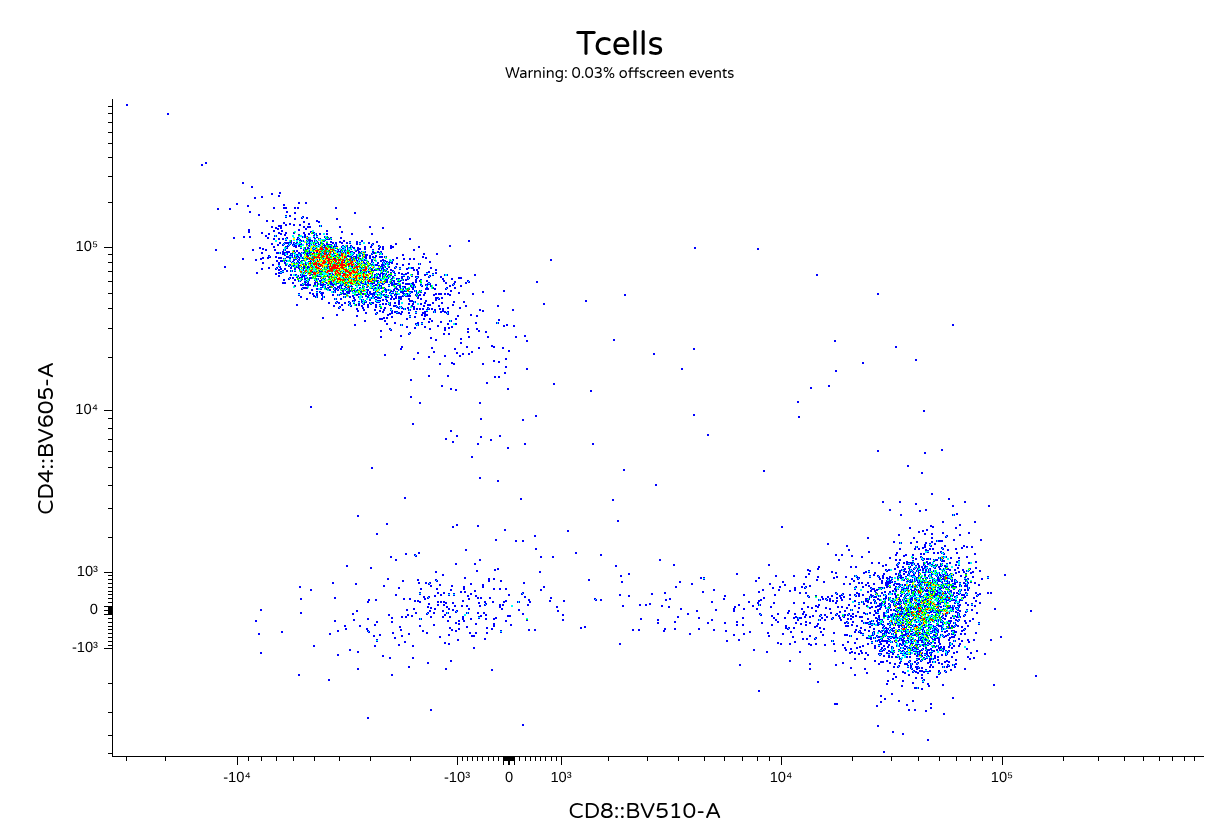
TRU-OLS

Take Away

In this walk-through, we showcased how to install Julia, activate TRU-OLS within a Positron project folder, and then leverage our existing knowledge about flow cytometry infrastructure as implemented in R via the flowWorkspace package to gather the required inputs. We then wrote a small helper and wrapper function to handoff these inputs to Julia for unmixing, before returning them to R for formatting and export out as .fcs files.

Obviously, this is an initial implementation, and several areas could use additional improvements. This entire process was single-threaded, and could benefit from parallel computing implementation to take advantage of most computers having multiple cores. Additionally, the use of JuliaCall as an intermediate introduces some lag as it gets reactivated on each iteration.

And this has only been checked on Cytek Aurora files, so its likely some changes need to be implemented for other manufacturers.

Regardless, as with all the course code, all the above is AGPL3-0 licensed, and you are free to customize it to your hearts content. We gladly welcome any modifications/contributions to make the above coding examples more robust in the future.

Hopefully, this lowers the barrier of entry, so that anyone interested in exploring how the TRU-OLS method of unmixing might differ for their own datasets is able to gnerate a quick example for evaluation.

Cheers! David

Additional Resources

Reducing Spreading: Removing the Impact of Irrelevant Dyes Improves Unmixed Flow Cytometry Data The original paper describing TRU-OLS, describing the methodology. If you are trying to customize the function further to take advantage of some of the non-default options, worth checking out.

Introduction to Julia for R users A blogpost by Nicola Rennie, covering some of the intro to Julia details that R users would appreciate knowing

Unmixing with Luciernaga The walk-through vignette documenting how to use the Luciernaga unmixing helper functions (still under development)