# Remove existing installation
remove.packages("flowGate")

# Install the new version
remotes::install_github("NKInstinct/flowGate") # If non-functional, try the class fork at "DavidRach/flowGate"Clean up Gates for Signature Retrieval



For the YouTube livestream recording, see here
For screen-shot slides, click here
Background
During weeks twelve through fourteen of the Cytometry in R course, we primarily focus on how to work with raw Spectral Flow Cytometry (SFC) .fcs files. During Week 12, we learn how to extract out and characterize fluorescent signatures that are present in our unmixing controls (both single-color and unstained). This is followed up on Week 13 by learning how to compare these signatures with each other, allowing us to predict how they will interact in context of a full SFC panel. Finally, in Week 14, we take the fluorescent signatures we have derived from our unmixing controls and use them to unmix full-stained samples.
Due to the Cytometry in R’s course use of GitHub, we are not able to include the full-sized .fcs files due to individual file size sharing constraints. The datasets used during Week’s 12 through 14 were consequently downsampled to get around this issue. However, working with the complete datasets can provide additional insight (as well as more closely replicate the experience of working with your own datasets). This walk-through therefore contains the steps needed to both retrieve and process the original .fcs files that were used from the ImmPort repository.
Continuing where we left off at the ImmPort walk-through, we will proceed to assemble GatingSets for the single-color unmixing controls (one for beads, and one for cells), as well as an additional GatingSet for the unstained unmixing controls. These will include clean-up gates to ensure we are only gating on events we are actually interested in. For a typical workflow, these would then be saved as their own GatingSet (.gs) object in your local environment as an intermediate step allowing for quick return. It is from these same intermediates that the final datasets for the Cytometry in R course’s Week 12-14 were retrieved from the final clean gate in each GatingSet using the Downsampling() function from Week 10.
Walk-Through
Planning
In the previous walk-through, we downloaded the original .fcs files for the SDY3080 dataset from ImmPort, focusing on the first two experiments (ILT_00 and ILT_01). We proceeded to save these within the data folder in their own respective subfolders based on the type of .fcs file (unmixing control bead or cell, unstained cell control, full-stained sample, etc.)
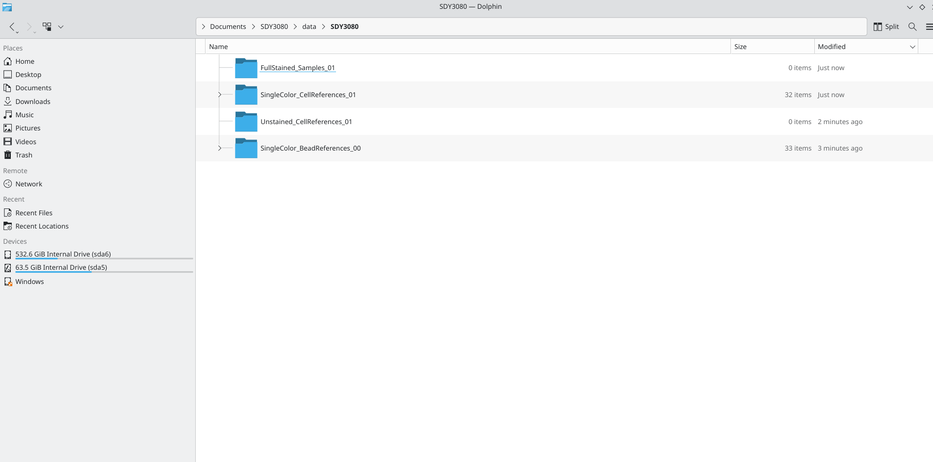
We will next load each of these subfolders into it’s own GatingSet object via the flowWorkspace package, and implement some basic cleanup gates using the flowGate package. We will then check the gates as applied to the individual specimens, ensuring that everything is in order before saving as an intermediate .gs object to allow for quick retrieval for subsequent data processing steps.
.gitignore
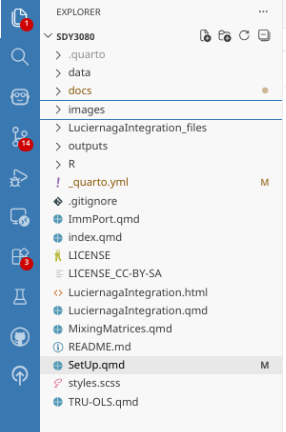
Before continuing, if you are working within your own project folder in Positron and are using version control, it would be useful to update your .gitignore file before proceeding to avoid acccidentally committing .fcs files that are too large for GitHub.
If a git repository has been initiated for your project folder, you can find your .gitignore file in the primary left-side bar. A .gitignore file is used to designate specific files or folders that should never be committed to Git. It is often used to avoid sending large files, sensitive information, or password files that you want to strictly remain on your local computer.
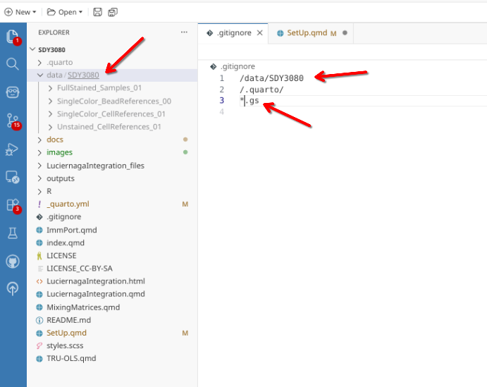
When opening for the first time, you will typically only have a couple items related to background Positron/Quarto processes listed. In the case of this walk-through, to ignore everything under data’s SDY3080 subfolder, I provided the “/data/SDY3080” value to the .gitignore file. Subsequently, anything in that folder is not tracked. Similarly, after the GatingSets get stored as .gs files to other locations outside that folder, I also want these to be ignored. Placing the line “*.gs” in the .gitignore file results in any file that ends in “.gs” is also ignored by version control, regardless of file.path.
Updating flowGate and Luciernaga
As you may recall, during Week 08 we explored how to use both the flowGate and openCyto packages to implement manual and automated gates. While using flowGate()’s Shiny app was quite helpful, we struggled with limited options in order to be able to adjust gates specifically for individual specimens, requiring the need to delete the entire gate and try again.
Since the flowGate package is open-source, I ended up writing several additional functions that allow for the adjustment of gate placement for individual specimens while leaving the same gate for the other specimens in place. I submitted these changes to the Andrew Wight, the package maintainer, who has merged them into the flowGate’s devel branch.
With the twice-yearly release cycle, this means they will roll into the regular Bioconductor version of flowGate in the next major release.
In the meanwhile, it is probably easiest to simply install flowGate via GitHub to take advantage of these new functions. As always, it is easier if you first remove the R package, close and reopen Positron, then install the new version.
The version containing both the ggplot2/ggcyto bug fixes as well as the new gating functions should be any version starting at/after 1.31.1
packageVersion("flowGate")[1] '1.13.1'Initial Setup
At this point, the workflow falls into routine that should be familiar to those who have gotten through the first section of the course. As always, start by loading the required R packages via the library() call.
library(flowWorkspace)As part of improvements to flowWorkspace, some behavior of
GatingSet objects has changed. For details, please read the section
titled "The cytoframe and cytoset classes" in the package vignette:
vignette("flowWorkspace-Introduction", "flowWorkspace")library(flowGate)Loading required package: ggcytoLoading required package: ggplot2Loading required package: flowCoreLoading required package: ncdfFlowLoading required package: BHRegistered polygon_gateRegistered span_gatelibrary(dplyr)
Attaching package: 'dplyr'The following object is masked from 'package:ncdfFlow':
filterThe following object is masked from 'package:flowCore':
filterThe following objects are masked from 'package:stats':
filter, lagThe following objects are masked from 'package:base':
intersect, setdiff, setequal, unionlibrary(purrr)Next, since we will be relying on the Downsampling() function that was created as part of Week 10 of the course, we can call the R folder in which it is stored to make it active in our local environment.
RFolder <- file.path("R")
MyFunctions <- list.files(RFolder, full.names=TRUE)
purrr::walk(.x=MyFunctions, .f=source)
With this done, we will need to designate both the input file.path (where our .fcs files are stored) as well as our output file.path (where we want any intermediate objects stored to). For the organization schema we had for this walk-through, this would look like
#StorageLocation <- file.path("course", "SDY3080", "data", "SDY3080")
StorageLocation <- file.path("data", "SDY3080")

#OutputLocation <- file.path("course", "SDY3080", "outputs")
OutputLocation <- file.path("outputs")
With these file paths set up, lets proceed to identify the individual subfolders where the different types of .fcs files are being stored, and designate them to their own respective variables for subsequent use.
Folders <- list.files(StorageLocation, full.names=TRUE)
Folders
[1] "data/SDY3080/FullStained_Samples_01"
[2] "data/SDY3080/SingleColor_BeadReferences_OO"
[3] "data/SDY3080/SingleColor_CellReferences_O1"
[4] "data/SDY3080/Unstained_CellReferences_O1" Samples_FullStained <- Folders[1] # Full-Stained # Don't Touch Yet
Beads_SC <- Folders[2] # Single-color Beads
Cells_SC <- Folders[3] # Single-color Cells
Cells_Unstained <- Folders[4] # Unstained CellsIndividual GatingSets
With the file paths set to the respective sub folders based on the type of .fcs file, lets proceed to load the .fcs files contained within each of them into their own respective GatingSet objects in our environment.
First up, lets create a “BeadsSC_GatingSet” for the bead single-color unmixing controls
# Beads Single Colors
Beads_files <- list.files(Beads_SC, pattern=".fcs",
 full.names=TRUE, recursive=TRUE)

BeadsSC_cytoset <- load_cytoset_from_fcs(Beads_files,
 truncate_max_range=FALSE, transformation=FALSE)

BeadsSC_GatingSet <- GatingSet(BeadsSC_cytoset)
BeadsSC_GatingSet
pData(BeadsSC_GatingSet)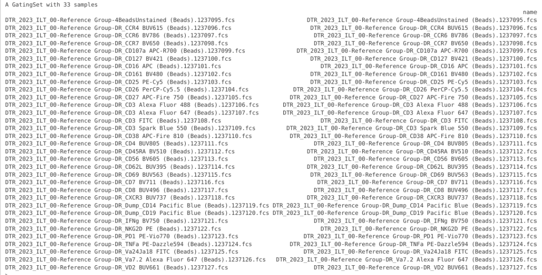
Next, a “CellsSC_GatingSet” for the cell single-color unmixing controls
# Cells Single Colors
CellsSC_files <- list.files(Cells_SC, pattern=".fcs",
 full.names=TRUE, recursive=TRUE)

CellsSC_cytoset <- load_cytoset_from_fcs(CellsSC_files,
 truncate_max_range=FALSE, transformation=FALSE)

CellsSC_GatingSet <- GatingSet(CellsSC_cytoset)
CellsSC_GatingSet
pData(CellsSC_GatingSet)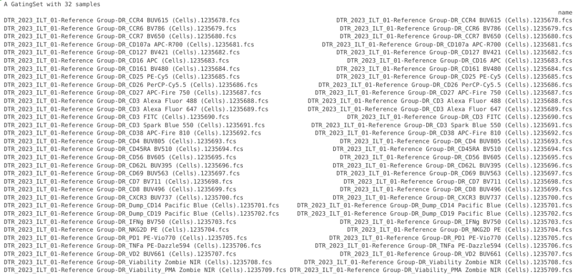
And last but not least, a “Unstained_GatingSet” for the unstained unmixing controls
# Cells Single Colors
Unstained_files <- list.files(Cells_Unstained, pattern=".fcs",
 full.names=TRUE, recursive=TRUE)

Unstained_cytoset <- load_cytoset_from_fcs(Unstained_files,
 truncate_max_range=FALSE, transformation=FALSE)

Unstained_GatingSet <- GatingSet(Unstained_cytoset)
Unstained_GatingSet
pData(Unstained_GatingSet)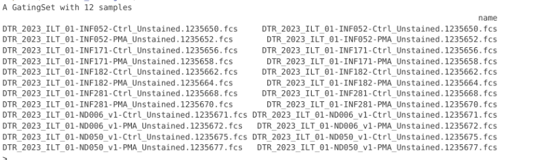
Transformation
In the next couple walk-throughs, we are working with raw .fcs files. You may be wondering if we need to transform these files? Since we will be working with extracting out the single-color and autofluorescence signatures, which rely on raw values, our first inclination would be correctly assume we do not need to transform, as this might impact the overall signature.
However, we first need to gate on cells that are positive for a given marker before we can extract the signature values from these cells. Since flow cytometry data for the fluorophores is typically visualized on a biexponential or logarithmic scale, this doesn’t work out very well in practice if we left the untransformed and viewed linearly. So we will need to first transform our datasets, but remember to use the “inverse.transform=TRUE” argument at the time of data retrieval to get back the original value from our gated cells.
SFC_Parameters <- colnames(BeadsSC_GatingSet)
FluorophoresOnly <- SFC_Parameters[!stringr::str_detect(SFC_Parameters, "FSC|SSC|Time")]

Biexponential <-  flowjo_biexp_trans(channelRange=4096, maxValue=4194304,
  pos=5.62, neg=0, widthBasis=-1000)
MyBiexTransform <- transformerList(FluorophoresOnly, Biexponential)
transform(BeadsSC_GatingSet, MyBiexTransform)
SFC_Parameters <- colnames(CellsSC_GatingSet)
FluorophoresOnly <- SFC_Parameters[!stringr::str_detect(SFC_Parameters, "FSC|SSC|Time")]
Biexponential <- flowjo_biexp_trans(channelRange=4096, maxValue=4194304,
pos=5.62, neg=0, widthBasis=-1000)
MyBiexTransform <- transformerList(FluorophoresOnly, Biexponential)
transform(CellsSC_GatingSet, MyBiexTransform)SFC_Parameters <- colnames(Unstained_GatingSet)
FluorophoresOnly <- SFC_Parameters[!stringr::str_detect(SFC_Parameters, "FSC|SSC|Time")]
Biexponential <- flowjo_biexp_trans(channelRange=4096, maxValue=4194304,
pos=5.62, neg=0, widthBasis=-1000)
MyBiexTransform <- transformerList(FluorophoresOnly, Biexponential)
transform(Unstained_GatingSet, MyBiexTransform)Initial Gates
Having set up our initial GatingSets, we will now add a few initial gates using the flowGate package, using the iteration table approach that was showcased back during Week 08. For beads, these gates will consist of a scatter and a singlets gate.
BeadGatingTable <- tibble::tribble(
  ~filterId,    ~dims,                          ~subset,
  "scatter",    list("FSC-A", "SSC-A"),      "root",
  "singlets",   list("FSC-A", "FSC-H"),          "scatter"
)
For the cells, since quite a few of the controls used cord blood mononuclear cells, we will include an additional gate to exclude any residual RBCs or pre-RBCs that might remain after freeze-thaw.
CellGatingTable <- tibble::tribble(
  ~filterId,    ~dims,                          ~subset,
  "singlets",   list("FSC-A", "FSC-H"),          "root",
  "nonRBCs",     list("SSC-A", "SSC-B-A"),    "singlets",
  "scatter",    list("FSC-A", "SSC-A"),      "nonRBCs",
)
Beads
To get started, we will run the following code block. The gs_apply_gating_strategy will allow us to draw the initial gates designated above in the template for an individual specimen.
flowGate::gs_apply_gating_strategy(BeadsSC_GatingSet, gating_strategy = BeadGatingTable)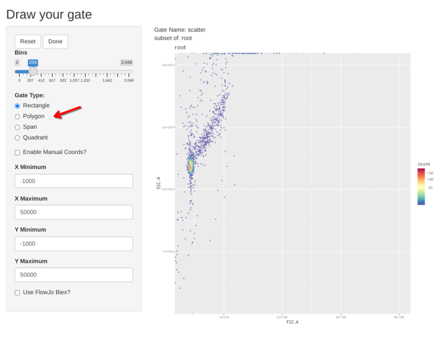
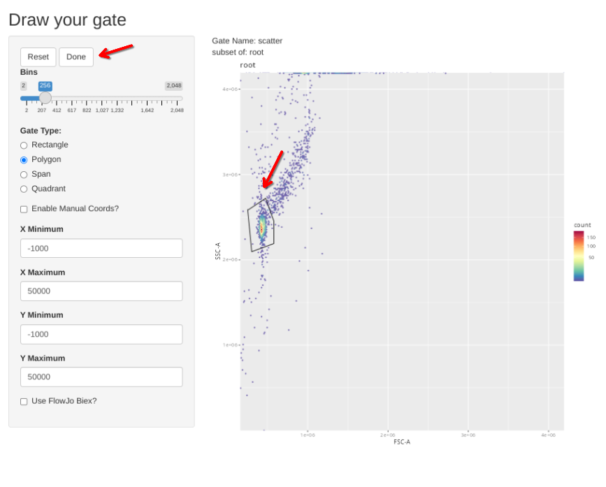
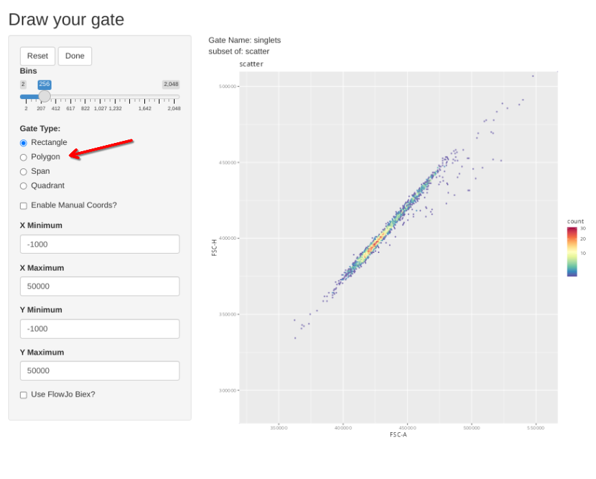
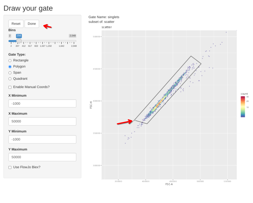
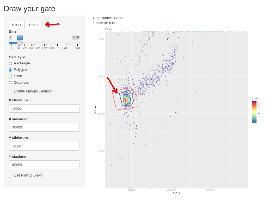
Subsequently, the new gs_apply_gate_check() function gets called for each of these newly created gates, allowing us to correct the gate if it did not correctly get applied to an individual specimen. We can do this first for the scatter gate
gs_apply_gate_check(gs=BeadsSC_GatingSet, gate="scatter")In a situation where the gate is good without any adjustments, simply click Done to move to the next specimen.
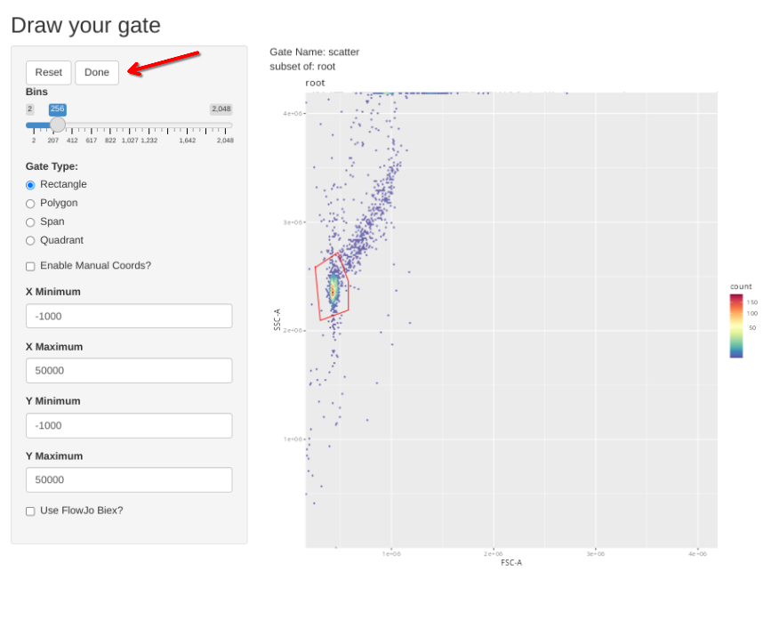
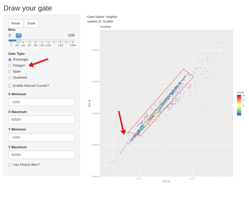
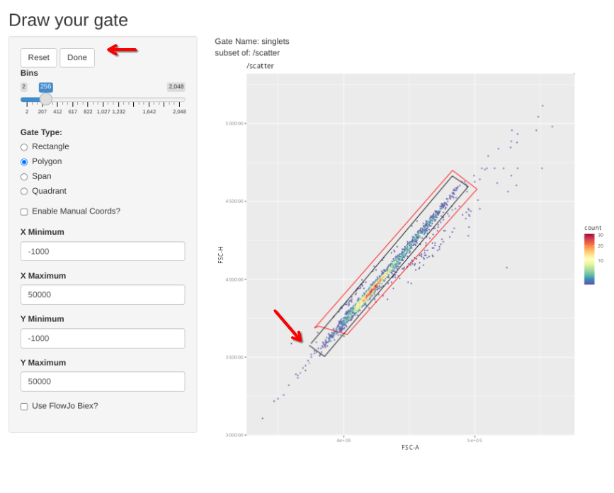
If however, you want to correct the gate, select polygon and proceed to draw a new one. If you mess up and want to redraw the gate, select Reset.
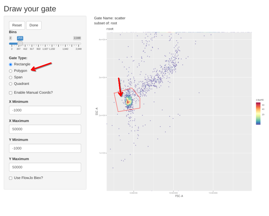
When the new gate is set, select Done to proceed to the next specimen.
And then proceed to the singlets gate and repeat the process
gs_apply_gate_check(gs=BeadsSC_GatingSet, gate="singlets")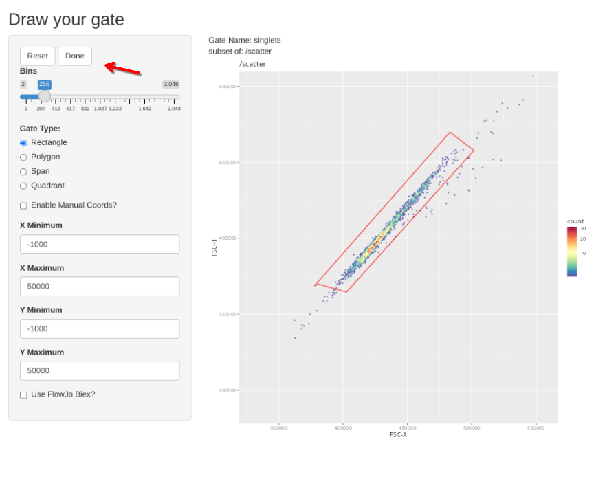
We can also use the new gs_to_openCyto to translate our drawn gates for a particular specimen out as a gatingTemplate.csv, allowing us to implement the exact same gates in the future with other specimens using the openCyto package.
gs_to_openCyto(gs=BeadsSC_GatingSet, sample=1, outpath=OutputLocation,
 filename = "BeadSetUpGates")
And last but not least, now that we have checked all these gates and verified/corrected that they are correct across all individuals, we can save these out as intermediate .gs object for later use.
BeadSaveHere <- file.path(OutputLocation, "BeadsSCs_GS.gs")

save_gs(BeadsSC_GatingSet, BeadSaveHere)
With the GatingSet for the bead single-color unmixing controls now set up, we can proceed to carry out the same steps for the cell single-color unmixing controls.
Cells - Single Colors
Similar to what we did for the beads, we will start off by running the gs_apply_gating_strategy to permit us to draw the initial gates designated n the template above for an individual specimen, which are subsequently applied to all specimens
flowGate::gs_apply_gating_strategy(CellsSC_GatingSet, gating_strategy = CellGatingTable)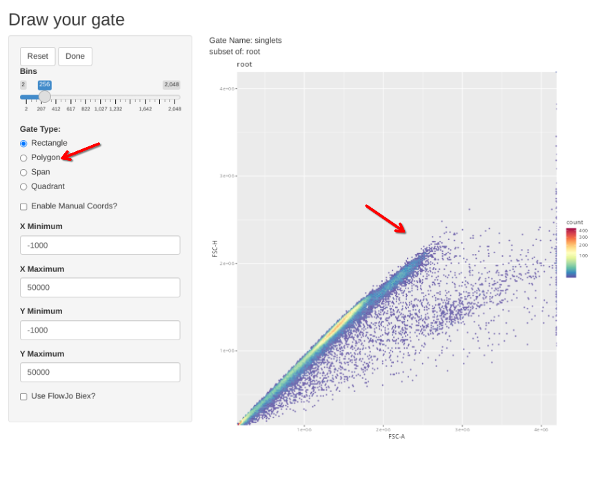
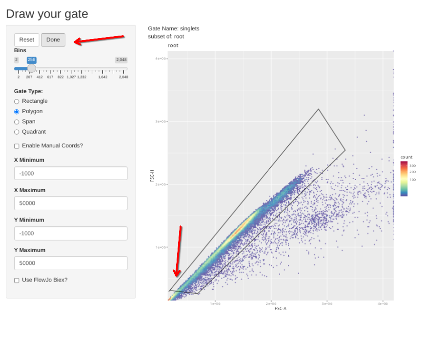
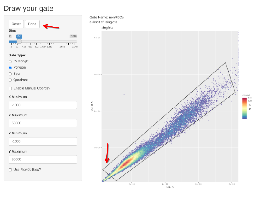
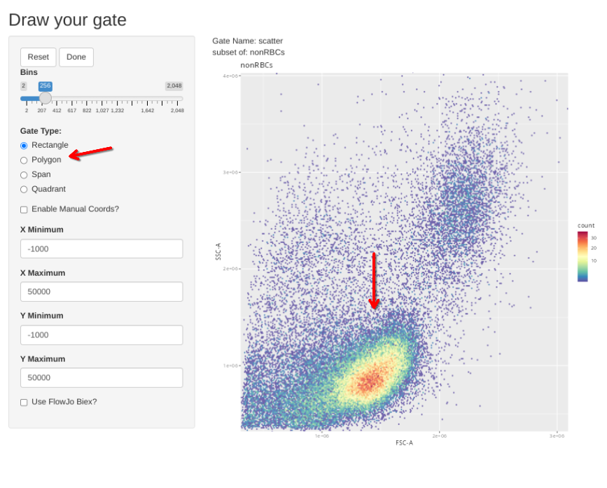
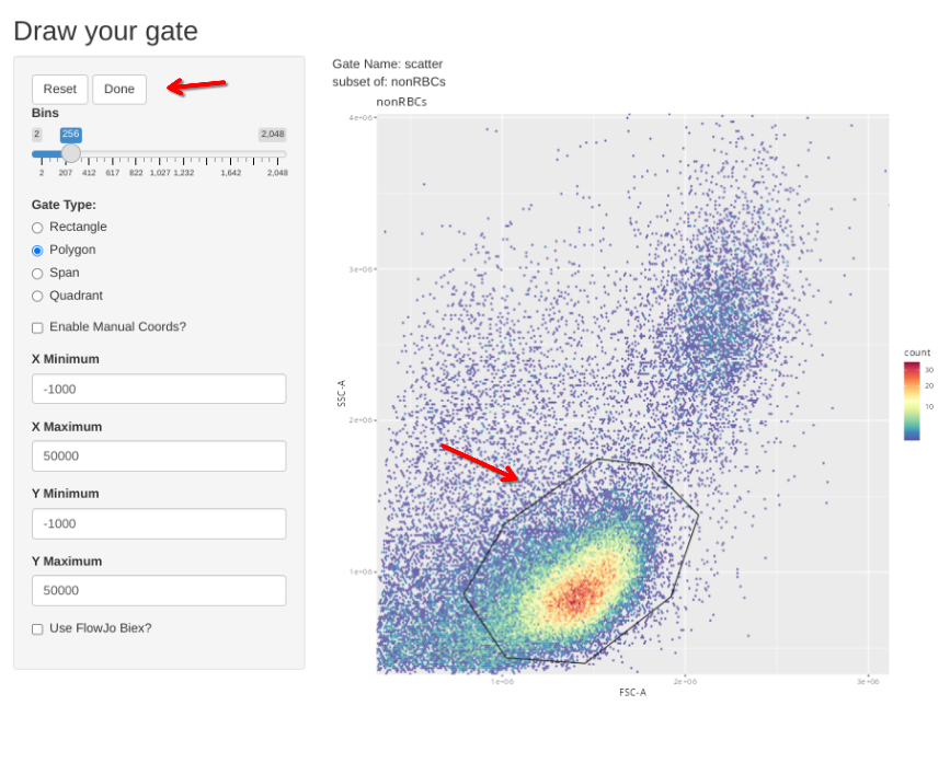
Subsequently, the new gs_apply_gate_check() function can be called for each of these newly created gates, allowing us to correct the gate if it did not correctly get applied to an individual specimen. We can do this first for the singlets gate
gs_apply_gate_check(gs=CellsSC_GatingSet, gate="singlets")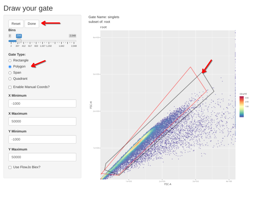
We can then follow up with checking the exclusion gate for RBCs
gs_apply_gate_check(gs=CellsSC_GatingSet, gate="nonRBCs")We can then wrap up with checking our scatter gate and adjusting as necessary (remembering we have some samples that are CBMC vs. PBMC, or PMA-ionomycin activated vs. control)
gs_apply_gate_check(gs=CellsSC_GatingSet, gate="scatter")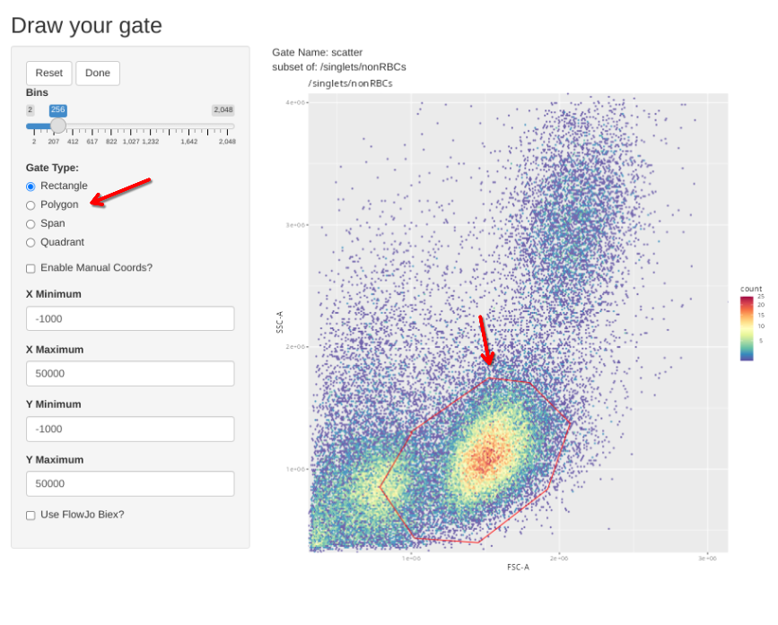
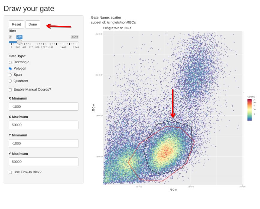
Additionally, we have a couple single-color controls where we need to adjust the scatter gate to a different location on the FSC x SSC plot. These include our single-color for CD14, where the brightest staining cells are going to be among the monocytes; and the two Zombie NIR controls, where the brightest cells are going to be among the dead cells between the debris and the healthy cells.
To save our eyesight (and sanity), we can use the pData() function to retrieve the metadata, and use the dplyr packages row_number() function alongside mutate() to quickly figure out the row for each specimen present.
pd <- pData(CellsSC_GatingSet)
pd |> mutate(Row = dplyr::row_number())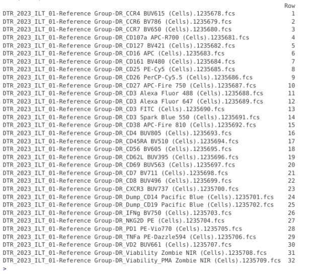
With the information we needed retrieved, we can then proceed the number designated within the [] to provide the proper GatingSet index, and then run gs_apply_gate_check() individually to adjust each of these single-color “scatter” gate exceptions.
gs_apply_gate_check(gs=CellsSC_GatingSet[24], gate="scatter") # Adjust to Monocytes # CD14 PacBlue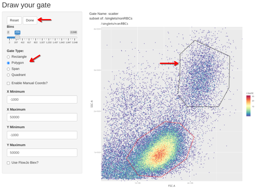
gs_apply_gate_check(gs=CellsSC_GatingSet[31], gate="scatter") # Adjust to Dead # Zombie NIR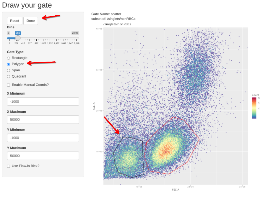
gs_apply_gate_check(gs=CellsSC_GatingSet[32], gate="scatter") # Adjust to Dead # Zombie NIR PMA-stimulated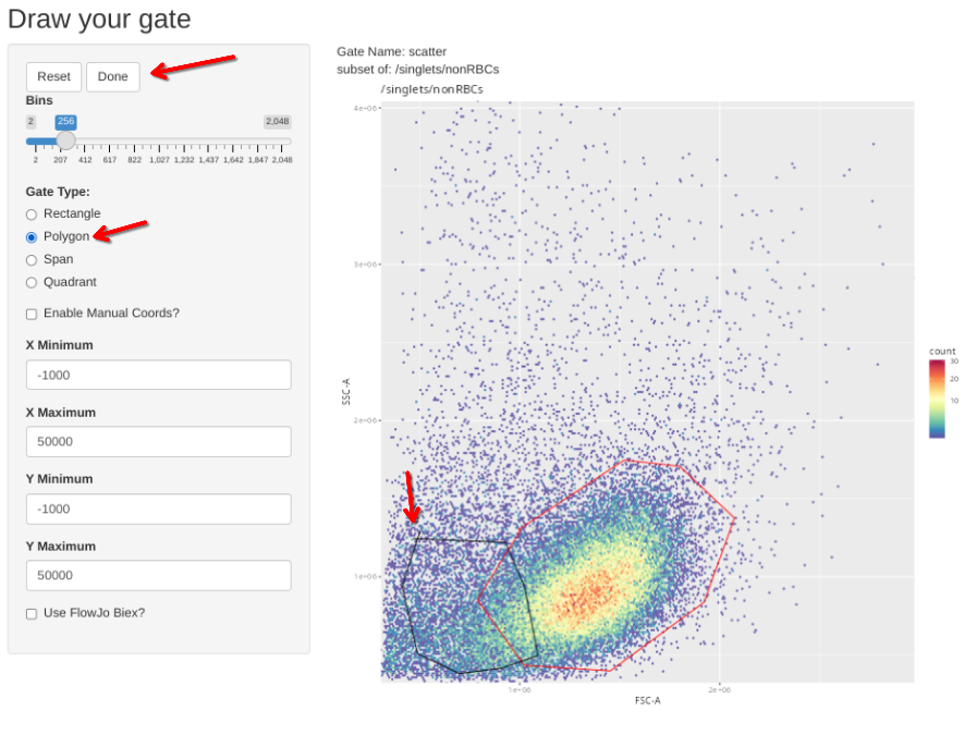
We can also use the new gs_to_openCyto to translate our drawn gates for a particular specimen out as a gatingTemplate.csv, allowing us to implement the exact same gates in the future with other specimens using the openCyto package.
gs_to_openCyto(gs=CellsSC_GatingSet, sample=1, outpath=OutputLocation,
 filename = "CellsSCs_SetUpGates")
And last but not least, now that we have checked all these gates and verified/corrected that they are correct across all individuals, we can save these out as intermediate .gs object for later use.
CellsSCSaveHere <- file.path(OutputLocation, "CellsSCs_GS.gs")

save_gs(CellsSC_GatingSet, CellsSCSaveHere)
Cells - Unstained
With the single-color GatingSets now set up for both the beads and cells, we can proceed to finish setting up the initial GatingSet for the unstained controls. For the SDY3080 dataset, unstained controls were acquired for each cord blood specimen, for both the control and PMA-ionomycin stimulated conditions (which may or may have not been a tad bit overkill in hindsight).
The process for setting up the initial gates is nearly identical as that of the single-color controls, with the main gate of importance for any adjustments being the scatter gate which will be different between the adult donor PBMC and CBMC specimens.
First, apply the initial gates
flowGate::gs_apply_gating_strategy(Unstained_GatingSet, gating_strategy = CellGatingTable)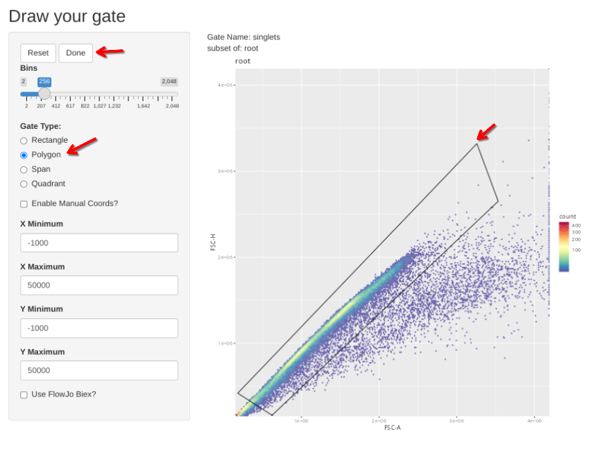
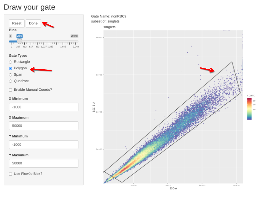
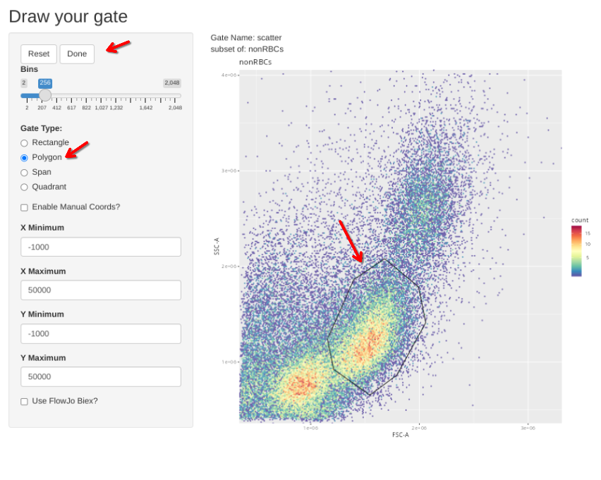
Then check the individual gates across individual specimens. Select Done if no change is needed, alternatively, select polygon, draw your gate, and then select Done to proceed to the next specimen.
gs_apply_gate_check(gs=Unstained_GatingSet, gate="singlets")gs_apply_gate_check(gs=Unstained_GatingSet, gate="nonRBCs")gs_apply_gate_check(gs=Unstained_GatingSet, gate="scatter")gs_to_openCyto(gs=Unstained_GatingSet, sample=1, outpath=OutputLocation,
filename = "CellsUnstained_SetUpGates")CellsUnstainedSaveHere <- file.path(OutputLocation, "CellsUnstained_GS.gs")
save_gs(Unstained_GatingSet, CellsUnstainedSaveHere)Downsampling
And finally, with all the clean-up gates properly applied to each of the three GatingSets, it was at this point of the workflow that I used the Downsampling() function we had created back during Week 10 to save out up to 5000 beads and 10000 cells for each of the controls for subsequent use as the Week 12 through Week 14 datasets. The example code can be seen below.
ClassFolder <- file.path(OutputLocation, "ClassDownsampled")

if (!dir.exists(ClassFolder)){dir.create(ClassFolder)}

SpecificFolder <- file.path(ClassFolder, "SingleColor_BeadReferences_OO")

if (!dir.exists(SpecificFolder)){dir.create(SpecificFolder)}

AllDNs <- purrr::map(.x=BeadsSC_GatingSet, subset="singlets", .f=Downsampling, DownsampleCount=5000, addon="",
  returnType="fcs", StorageLocation=SpecificFolder, inverse.transform=TRUE)
ClassFolder <- file.path(OutputLocation, "ClassDownsampled")
if (!dir.exists(ClassFolder)){dir.create(ClassFolder)}
SpecificFolder <- file.path(ClassFolder, "SingleColor_CellReferences_O1")
if (!dir.exists(SpecificFolder)){dir.create(SpecificFolder)}
AllDNs <- purrr::map(.x=CellsSC_GatingSet, subset="scatter", .f=Downsampling, DownsampleCount=10000, addon="",
returnType="fcs", StorageLocation=SpecificFolder, inverse.transform=TRUE)ClassFolder <- file.path(OutputLocation, "ClassDownsampled")
if (!dir.exists(ClassFolder)){dir.create(ClassFolder)}
SpecificFolder <- file.path(ClassFolder, "Unstained_CellReferences_O1")
if (!dir.exists(SpecificFolder)){dir.create(SpecificFolder)}
AllDNs <- purrr::map(.x=Unstained_GatingSet, subset="scatter", .f=Downsampling, DownsampleCount=10000, addon="",
returnType="fcs", StorageLocation=SpecificFolder, inverse.transform=TRUE)Take-Away
During this walk-through, we have loaded in our unmixing controls (both single-color and unstained) into their own respective GatingSets, transformed and applied initial gates. We in turn using the new flowGate functions double checked and validated these initial gate placements across each individual, modifying the individually applied gates as necessary, ensuring that everything was correctly applied before saving the GatingSets as intermediate .gs for future use. Hopefully, this will payoff further downstream in the analysis by limiting the effect that antibody aggregates, debris, doublets and dead cells end up getting selected along with cells of interest may have on the final derived signatures.
In the next portion of this walk-through, we will orchestrate the creation of individual gates for every single-color in our panel, allowing for the derivation of the single-color unmixing matrix that is needed to retrieve the normalized fluorescent signatures, as well as later on for use in unmixing the full-stained controls.

Additional Resources