#' Coereba Package Internal, used for Utility_Behemoth
#'
#' @param plot The ggplot2 object
#' @param Method Passed method for statistics
#' @param ThePData Dataframe containing index and pvalues
#' @param SingleY The derrived height at which to place the lines
#'
#' @importFrom dplyr select filter pull
#' @importFrom stringr str_wrap
#' @importFrom ggplot2 ggplot aes geom_boxplot scale_shape_manual
#' scale_fill_manual labs theme_bw element_blank element_text theme
#' geom_line geom_text scale_y_continuous lims
#' @importFrom ggbeeswarm geom_beeswarm
#' @importFrom tibble tibble
#' @importFrom scales percent
#'
#' @return Updated ggplot2 plot with stat lines
#'
#' @noRd
LineAddition <- function(plot, Method, ThePData, SingleY){
if (!is.null(ThePData)){
if (nrow(ThePData) > 0){
IndexSlots <- ThePData |> dplyr::pull(Index)
} else {IndexSlots <- NULL}
} else {IndexSlots <- NULL}
if (!is.null(IndexSlots)){
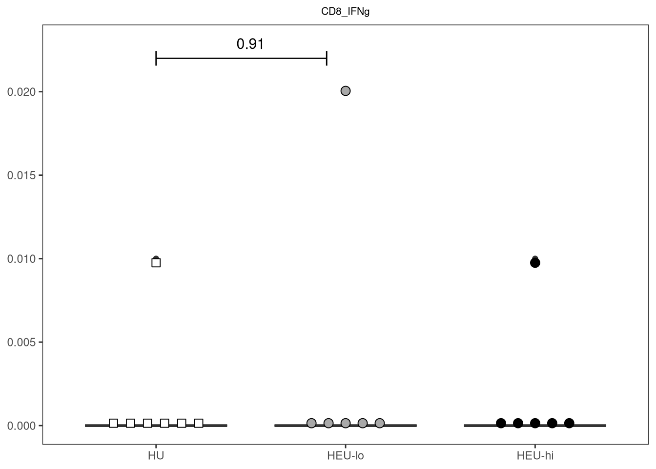
if (length(IndexSlots) < 3 & Method %in% c("Pairwise t-test", "Pairwise Wilcox test")){
Index1 <- ThePData |> dplyr::filter(Index == 1)
Index2 <- ThePData |> dplyr::filter(Index == 2)
Index3 <- ThePData |> dplyr::filter(Index == 3)
if (nrow(Index1) > 0){
FirstY <- SingleY*1
FirstP <- ThePData |> dplyr::filter(Index == 1) |> dplyr::pull(ThePvalues)
plot <- plot +
geom_line(data=tibble(x=c(1,1.9), y=c(FirstY, FirstY)), aes(x=x, y=y), inherit.aes = FALSE) +
geom_line(data=tibble(x=c(1,1), y=c(FirstY*0.98,FirstY*1.02)), aes(x=x, y=y), inherit.aes = FALSE) +
geom_line(data=tibble(x=c(1.9,1.9), y=c(FirstY*0.98,FirstY*1.02)),aes(x=x, y=y), inherit.aes = FALSE) +
geom_text(data=tibble(x=1.5, y=FirstY*1.04), aes(x=x, y=y, label = FirstP),size = 4, inherit.aes = FALSE)
}
if (nrow(Index2) > 0){
SecondY <- SingleY*1.1
SecondP <- ThePData |> dplyr::filter(Index == 2) |> dplyr::pull(ThePvalues)
plot <- plot +
geom_line(data=tibble(x=c(1,3), y=c(SecondY, SecondY)), aes(x=x, y=y), inherit.aes = FALSE) +
geom_line(data=tibble(x=c(1,1), y=c(SecondY*0.98,SecondY*1.02)), aes(x=x, y=y), inherit.aes = FALSE) +
geom_line(data=tibble(x=c(3,3), y=c(SecondY*0.98,SecondY*1.02)), aes(x=x, y=y), inherit.aes = FALSE) +
geom_text(data=tibble(x=2, y=SecondY*1.04), aes(x=x, y=y, label = SecondP), size = 4, inherit.aes = FALSE)
}
if (nrow(Index3) > 0){
ThirdY <- SingleY*1
ThirdP <- ThePData |> dplyr::filter(Index == 3) |> dplyr::pull(ThePvalues)
plot <- plot + geom_line(data=tibble(x=c(2.1,3), y=c(ThirdY, ThirdY)),aes(x=x, y=y), inherit.aes = FALSE) +
geom_line(data=tibble(x=c(2.1,2.1), y=c(ThirdY*0.98,ThirdY*1.02)), aes(x=x, y=y), inherit.aes = FALSE) +
geom_line(data=tibble(x=c(3,3), y=c(ThirdY*0.98,ThirdY*1.02)), aes(x=x, y=y), inherit.aes = FALSE) +
geom_text(data=tibble(x=2.55, y=ThirdY*1.04), aes(x=x, y=y, label = ThirdP), size = 4, inherit.aes = FALSE)
}
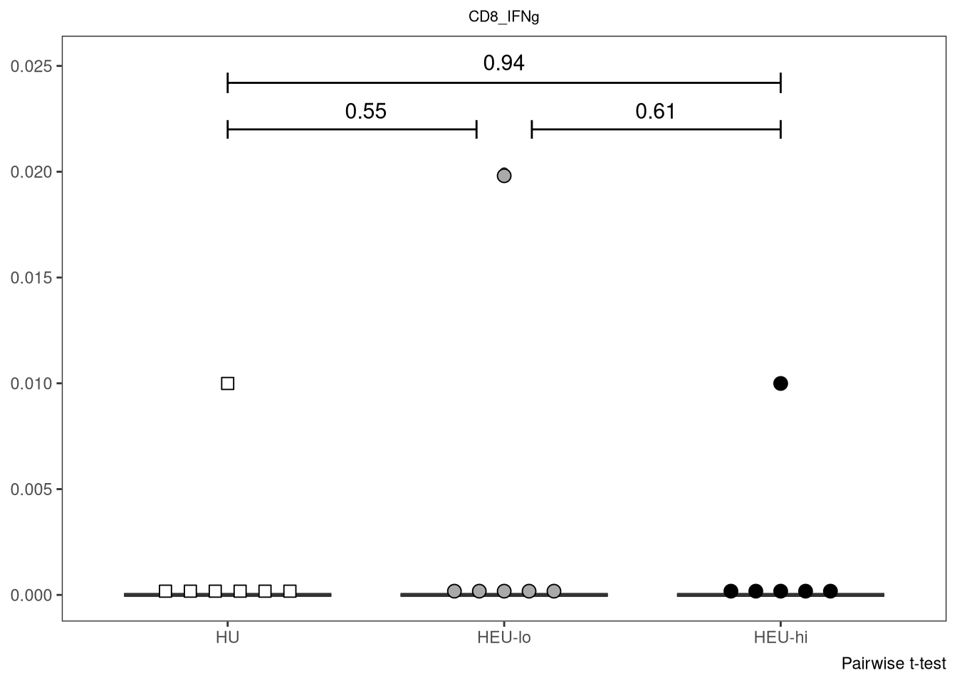
} else if (length(IndexSlots) == 3 & Method %in% c("Pairwise t-test", "Pairwise Wilcox test")){
FirstP <- ThePData |> dplyr::filter(Index == 1) |> dplyr::pull(ThePvalues)
SecondP <- ThePData |> dplyr::filter(Index == 2) |> dplyr::pull(ThePvalues)
ThirdP <- ThePData |> dplyr::filter(Index == 3) |> dplyr::pull(ThePvalues)
FirstY <- SingleY*1
SecondY <- SingleY*1.1
ThirdY <- SingleY*1
plot <- plot +
geom_line(data=tibble(x=c(1,1.9), y=c(FirstY, FirstY)), aes(x=x, y=y), inherit.aes = FALSE) +
geom_line(data=tibble(x=c(1,1), y=c(FirstY*0.98,FirstY*1.02)), aes(x=x, y=y), inherit.aes = FALSE) +
geom_line(data=tibble(x=c(1.9,1.9), y=c(FirstY*0.98,FirstY*1.02)),aes(x=x, y=y), inherit.aes = FALSE) +
geom_text(data=tibble(x=1.5, y=FirstY*1.04), aes(x=x, y=y, label = FirstP),size = 4, inherit.aes = FALSE) +
geom_line(data=tibble(x=c(2.1,3), y=c(ThirdY, ThirdY)),aes(x=x, y=y), inherit.aes = FALSE) +
geom_line(data=tibble(x=c(2.1,2.1), y=c(ThirdY*0.98,ThirdY*1.02)), aes(x=x, y=y), inherit.aes = FALSE) +
geom_line(data=tibble(x=c(3,3), y=c(ThirdY*0.98,ThirdY*1.02)), aes(x=x, y=y), inherit.aes = FALSE) +
geom_text(data=tibble(x=2.55, y=ThirdY*1.04), aes(x=x, y=y, label = ThirdP), size = 4, inherit.aes = FALSE) +
geom_line(data=tibble(x=c(1,3), y=c(SecondY, SecondY)), aes(x=x, y=y), inherit.aes = FALSE) +
geom_line(data=tibble(x=c(1,1), y=c(SecondY*0.98,SecondY*1.02)), aes(x=x, y=y), inherit.aes = FALSE) +
geom_line(data=tibble(x=c(3,3), y=c(SecondY*0.98,SecondY*1.02)), aes(x=x, y=y), inherit.aes = FALSE) +
geom_text(data=tibble(x=2, y=SecondY*1.04), aes(x=x, y=y, label = SecondP), size = 4, inherit.aes = FALSE) +
labs(caption = Method)
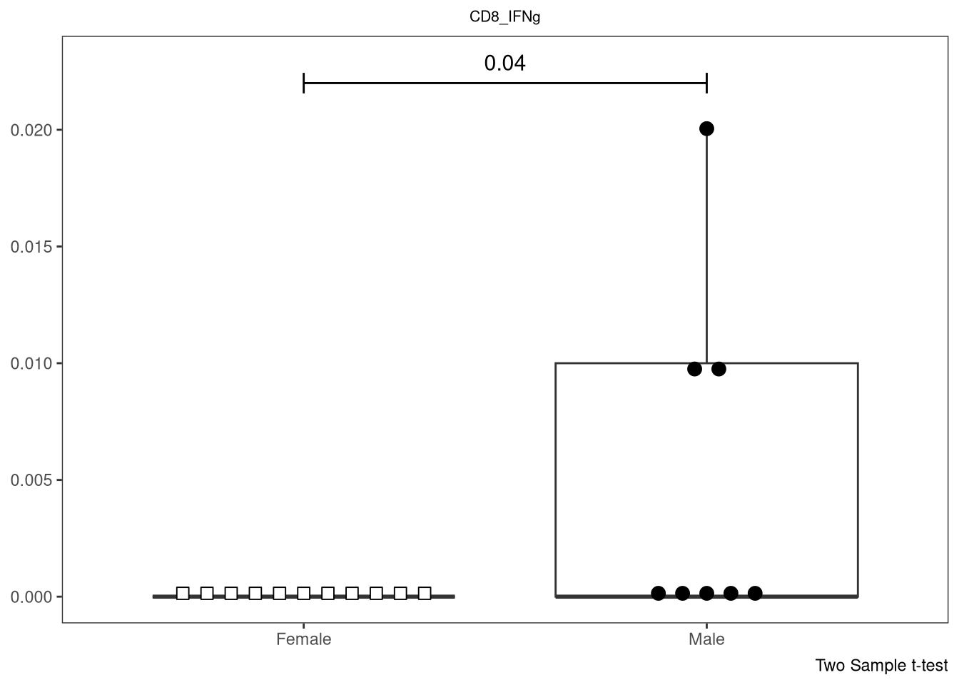
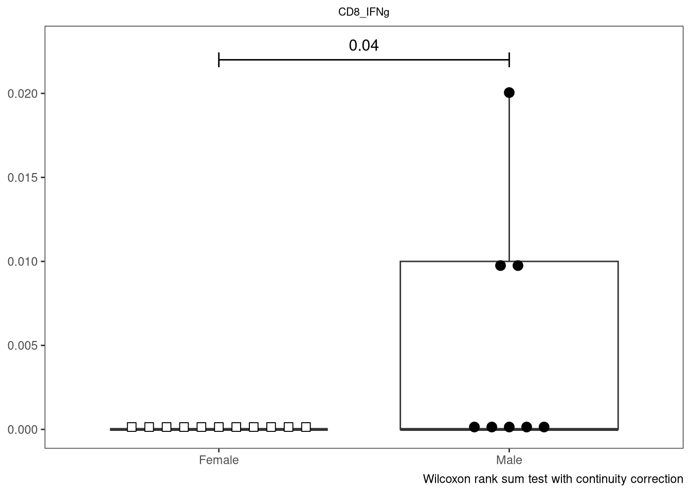
} else if (length(IndexSlots) == 1 & Method %in% c("Two Sample t-test",
"Wilcoxon rank sum test with continuity correction", "Wilcoxon rank sum exact test")){
SingleP <- ThePData |> pull(ThePvalues)
plot <- plot + geom_line(data=tibble(x=c(1,2), y=c(SingleY, SingleY)), aes(x=x, y=y), inherit.aes = FALSE) +
geom_line(data=tibble(x=c(1,1), y=c(SingleY*0.98,SingleY*1.02)), aes(x=x, y=y), inherit.aes = FALSE) +
geom_line(data=tibble(x=c(2,2), y=c(SingleY*0.98,SingleY*1.02)), aes(x=x, y=y), inherit.aes = FALSE) +
geom_text(data=tibble(x=1.5, y=SingleY*1.04), aes(x=x, y=y, label = SingleP), size = 4, inherit.aes = FALSE) +
labs(caption = Method)
} else if (length(IndexSlots) == 1 & Method %in% c("One-way Anova", "Kruskal-Wallis rank sum test")){
SingleP <- ThePData |> pull(ThePvalues)
plot <- plot + geom_line(data=tibble(x=c(1,3), y=c(SingleY, SingleY)), aes(x=x, y=y), inherit.aes = FALSE) +
geom_line(data=tibble(x=c(1,1), y=c(SingleY*0.98,SingleY*1.02)), aes(x=x, y=y), inherit.aes = FALSE) +
geom_line(data=tibble(x=c(3,3), y=c(SingleY*0.98,SingleY*1.02)), aes(x=x, y=y), inherit.aes = FALSE) +
geom_text(data=tibble(x=2, y=SingleY*1.04), aes(x=x, y=y, label = SingleP), size = 4, inherit.aes = FALSE) +
labs(caption = Method)
} else {return(plot)}
} else {return(plot)}
return(plot)
}


