Using Floreada

![]()
![]()
For the YouTube livestream recording, see here
For screen-shot slides, click here
Background
As a “Cytometry in R” course, we will primarily be working in R. However, within our daily workflows and projects here at our flow cytometry core, we often use various flow cytometry softwares (like FlowJo or FCS Express) for various tasks. Fortunately, R packages like CytoML can allow us to import our manually drawn gates from existing FlowJo workspaces so that we can work with them in R.
For this course, we are adamant about staying neutral in regards to both commercial software or instrument vendors as much as possible. If they have worked with the open-source community to make their files readable and accessible via R, we will showcase how to integrate those tools into your own workflows. At the same time, this being a free course, it doesn’t make sense to turn around and ask you to go and either free trial or buy an expensive software license just to see how a particular free R package works.
Fortunately, for showing how to use this CytoML functionality, we can use Floreada.io. It is a simple (but free) web-based analysis platform that can be used to draw manual gates for your .fcs files of interest. These can then be saved as Floreada workspaces for later use. We typically recommend it to users from labs that do flow experiments infrequently. Fortunately thanks to the hard work of its developers, it can also save the gated files as FlowJo v10 .wsp files, which with a small workaround become usable within the CytoML pipeline.
To facilitate this, we will provide a small walk-through of how to use it for those who want to create a .wsp with their own .fcs files for Week 5.
Walk-through
Floreada
Loading Dataset
First, open your web browser and navigate to the website
Click on Start to proceed to the next page.
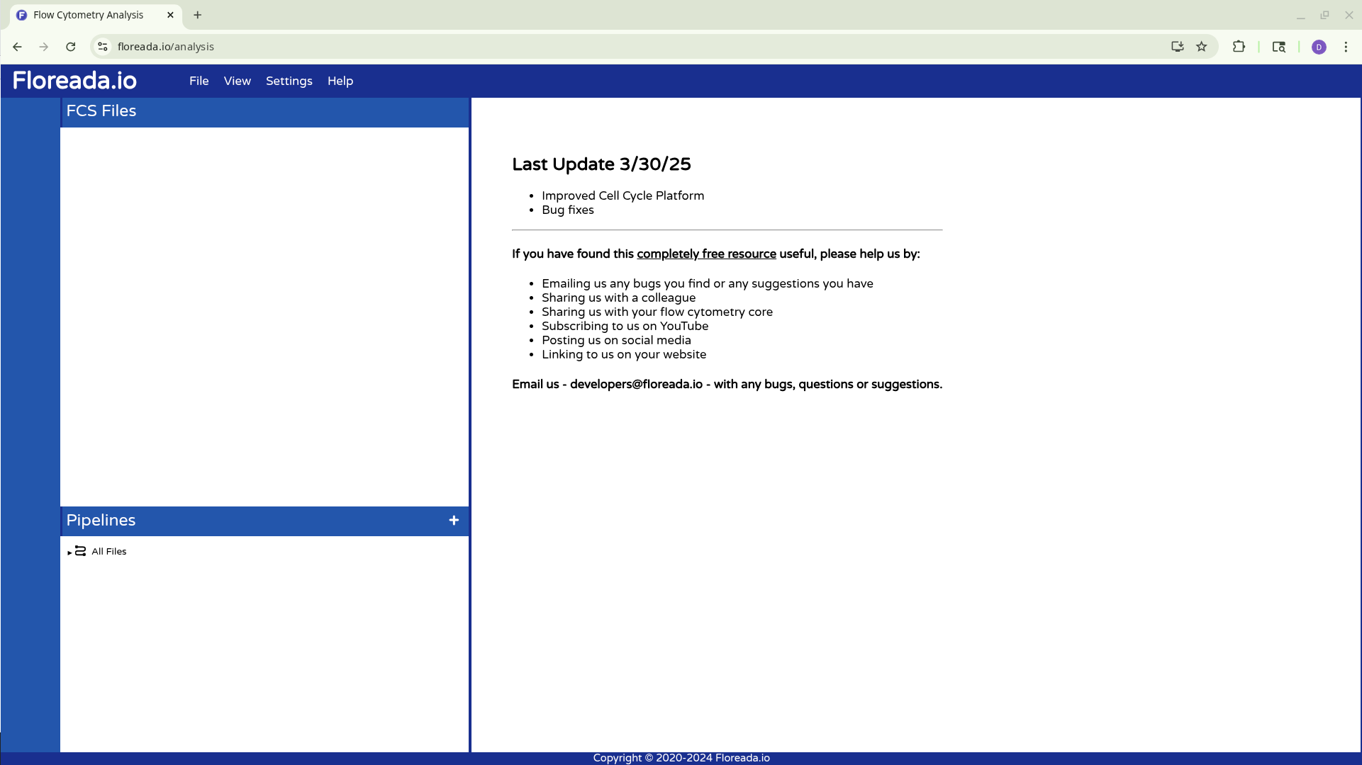
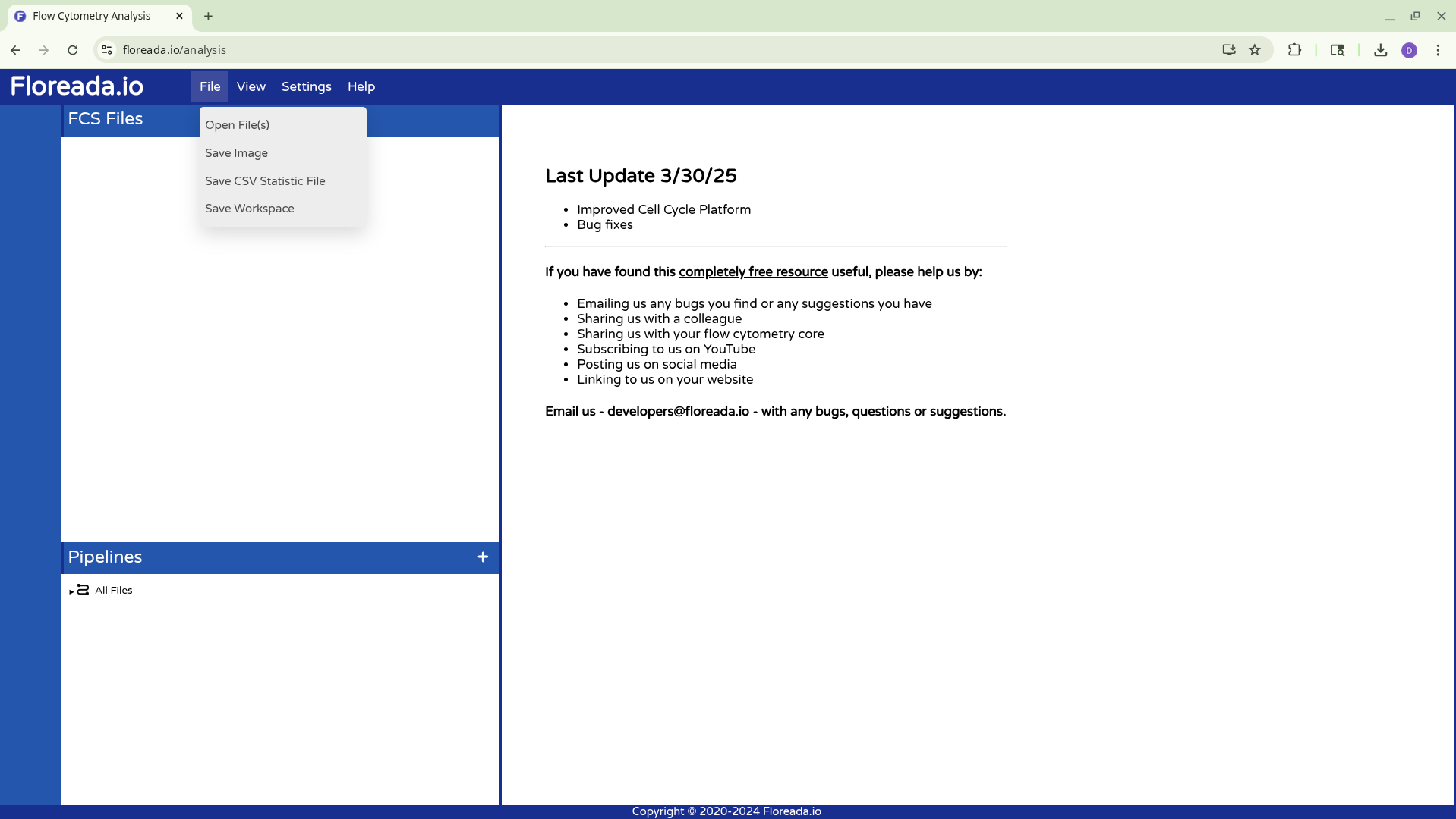
Once that is done, select the File tab on the upper navigation bar. Then click on Open File(s).

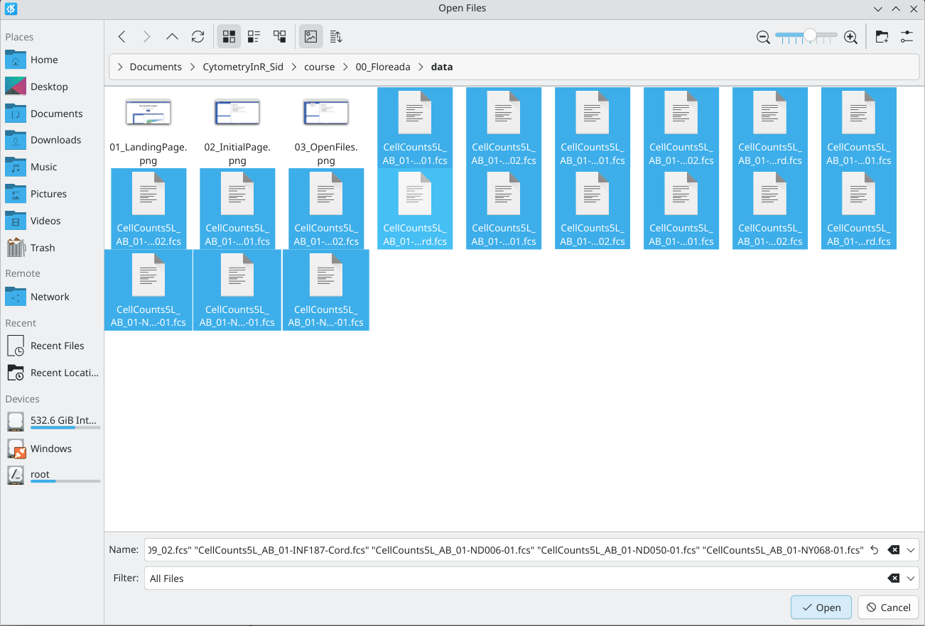
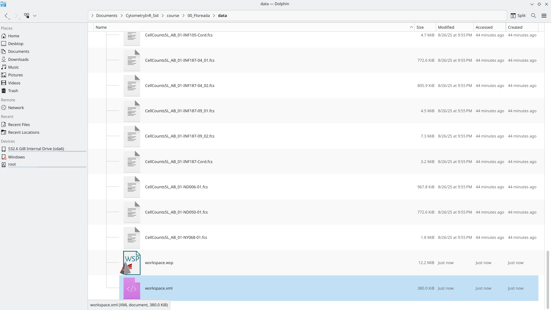
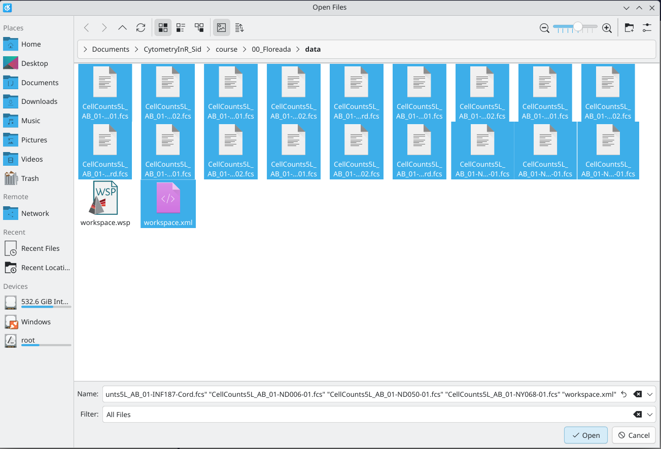
From there, select your .fcs files of interest, and click Open.
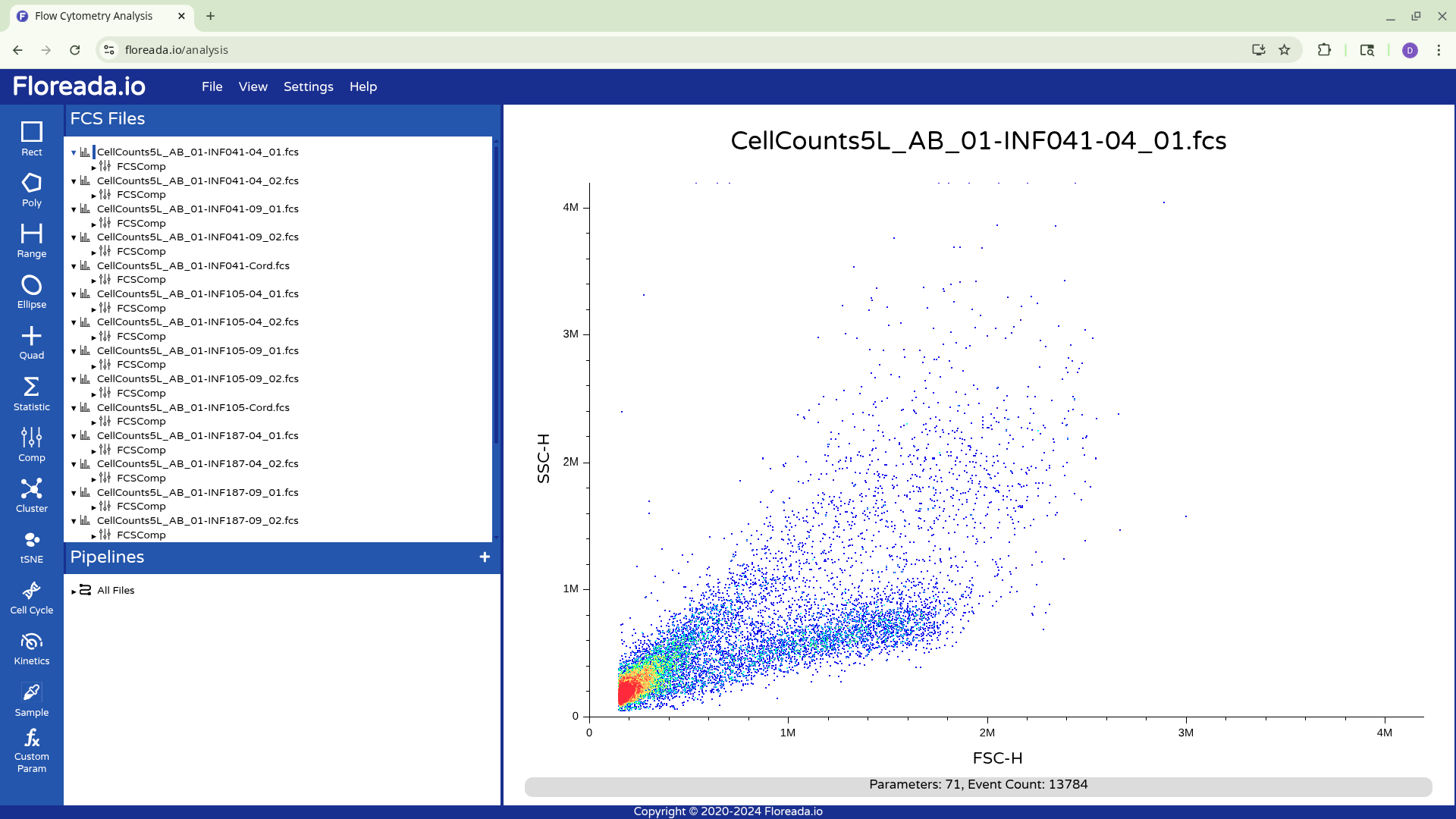
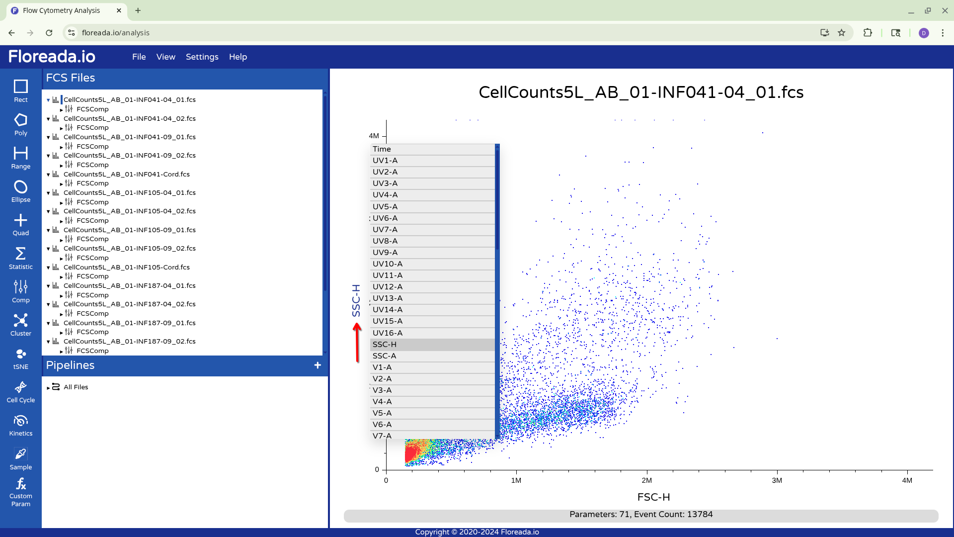
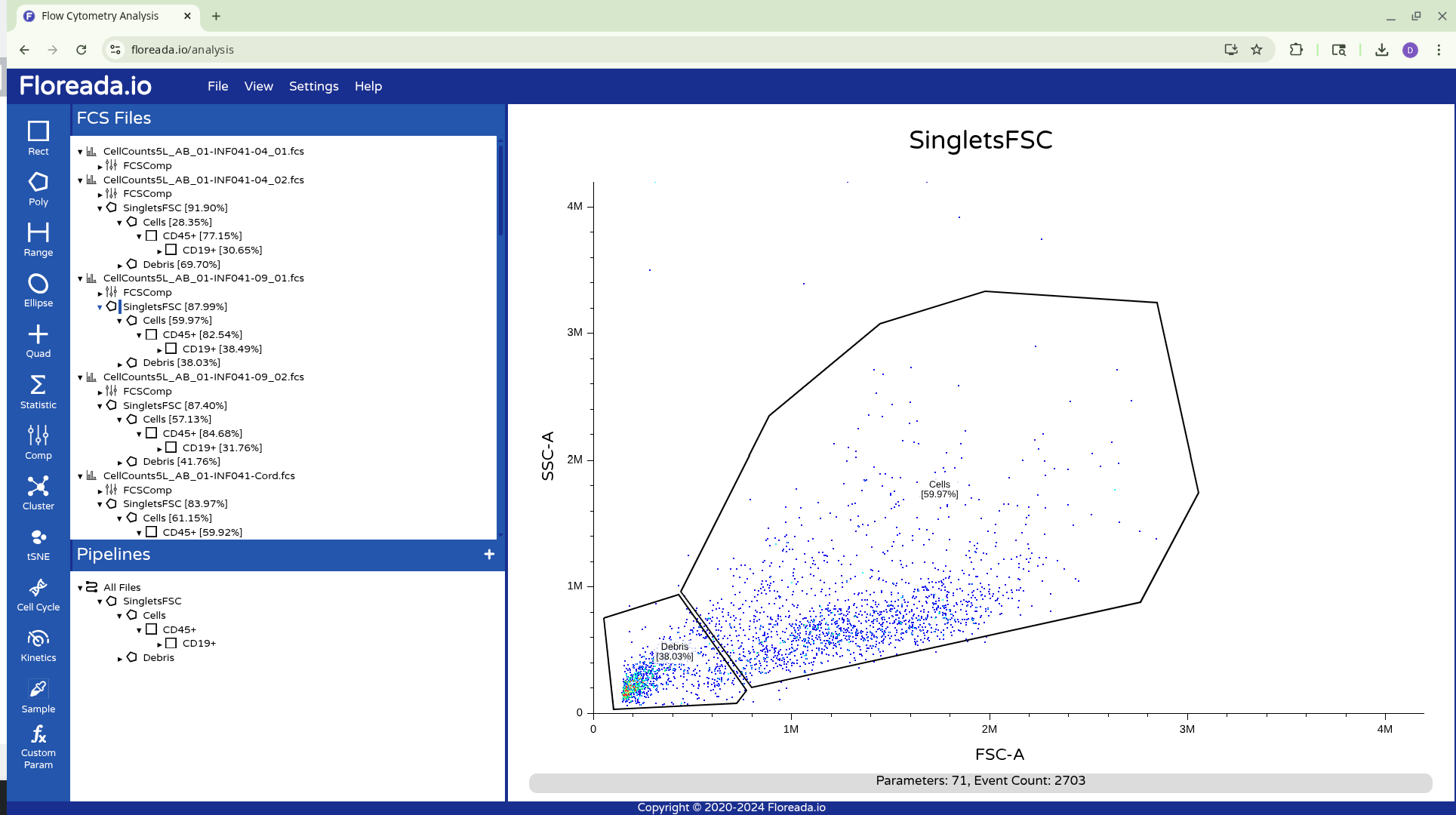
The .fcs files will now load in, and you should see a view similar to the one below. On the left side-bar, you have your gating options (Rectangle, Polygon, Range, Elipse, Quad, etc). Next to these on the right you have the FCS files that are loaded into the workspace. Then on the right, you have the visual display for your selected specimen.
Switching Axis Markers
If you left click on the axis name (SSC-H or FSC-H in this case), you will be able to select other markers by which to gate your specimen. For the provided example, we were using a raw spectral flow cytometry .fcs file, so the names of the detectors are present.
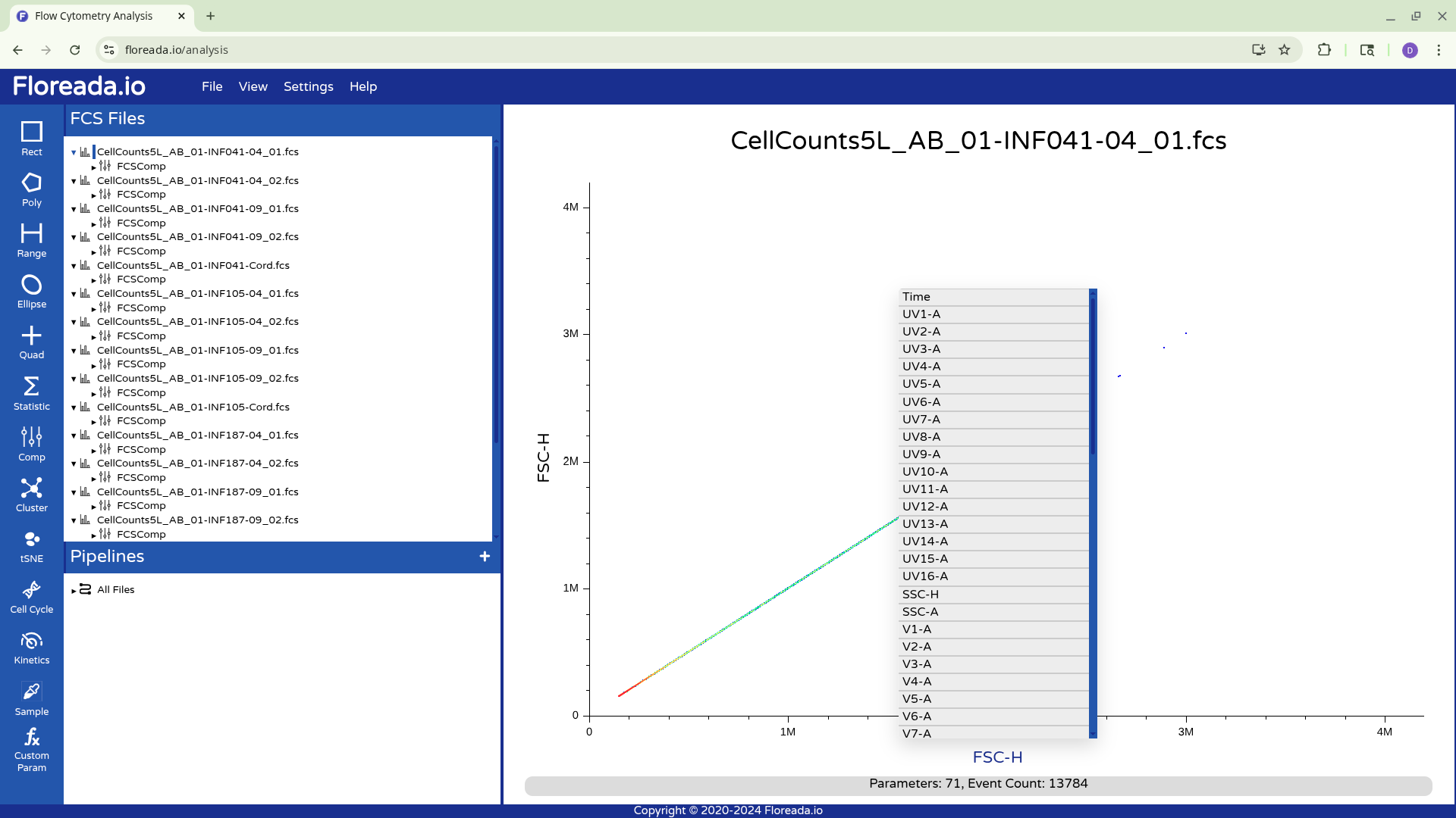
For now, I plan to start off by gating for singlets. I switch the y-axis to FSC-H, and then proceed to switch the x-axis to FSC-A.
Creating Gates
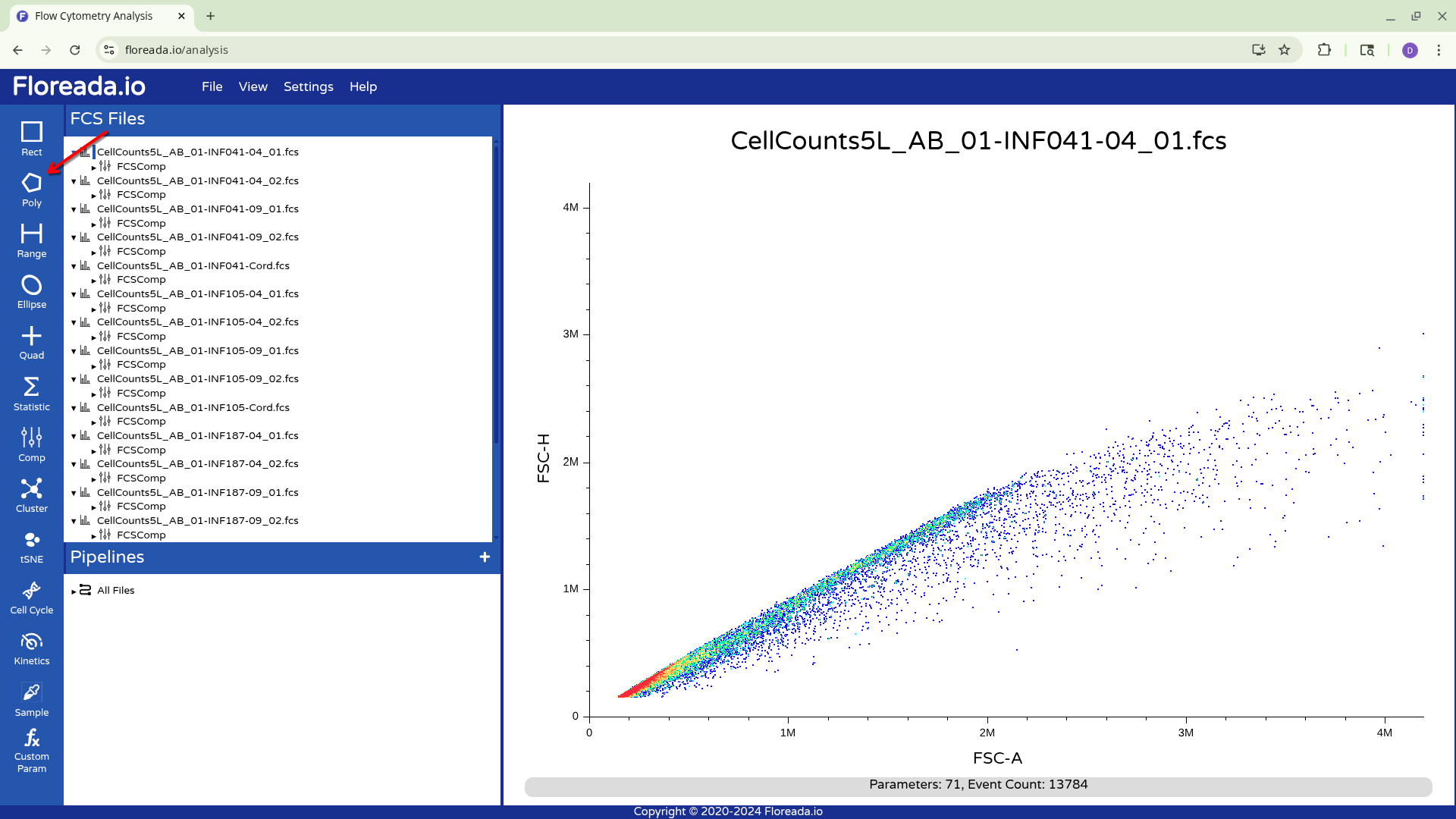
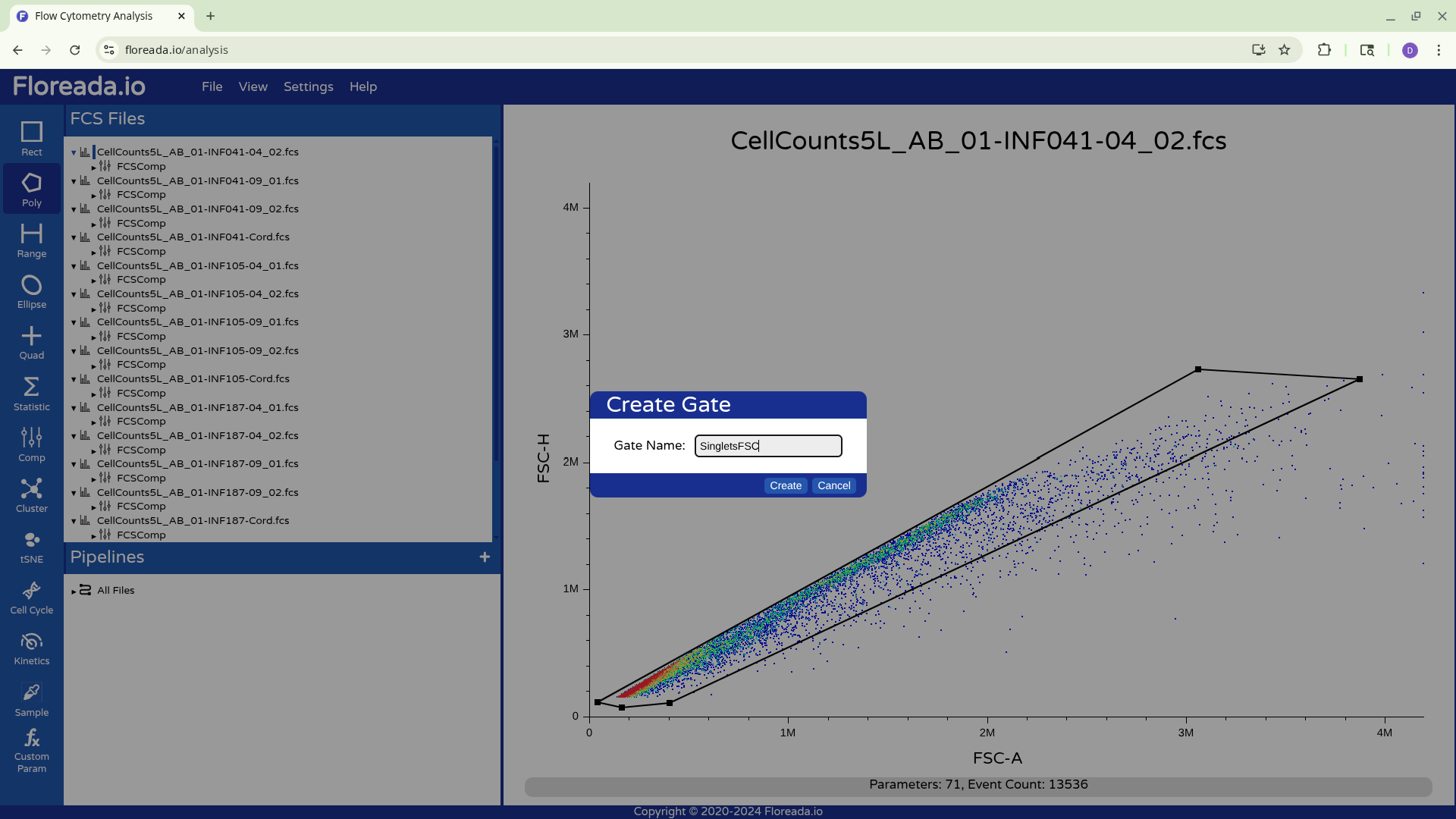
With this done, I can now select the Poly gate tab on the upper left.
Then manually click on the locations on the plot to add the individual gate nodes.
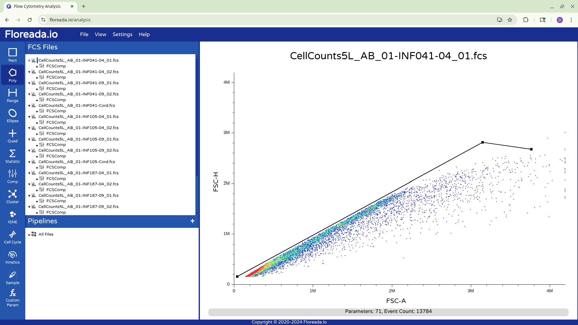
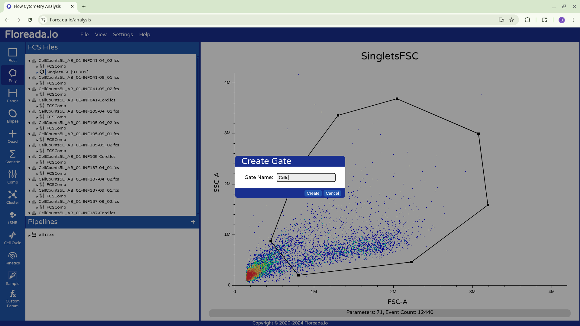
To complete the gate, I click back to the original node point. At this point, the popup will allow you to name the gate.
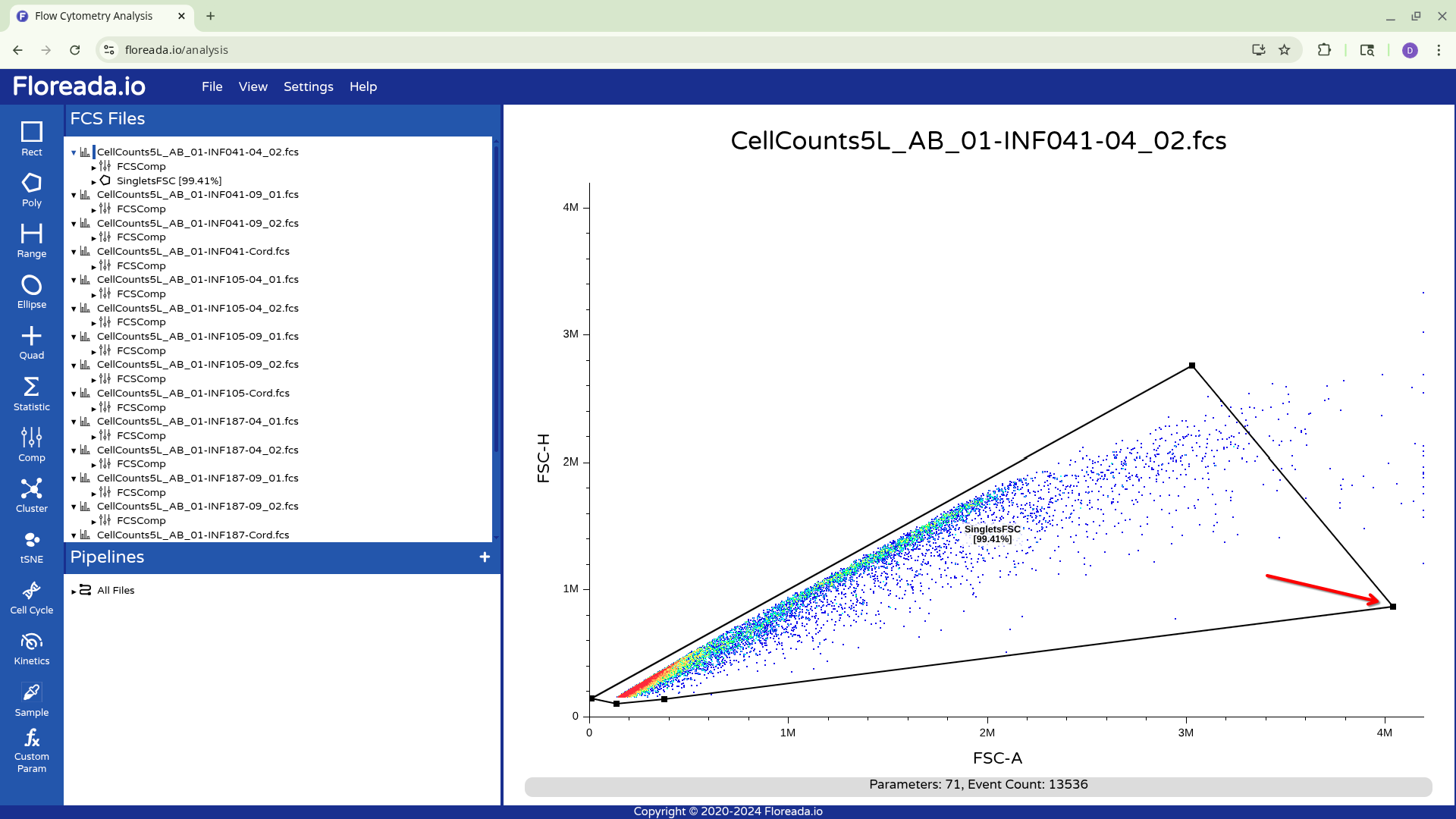
To adjust the polygon gate, you can click on a node and drag it to expand or contract in a particular direction
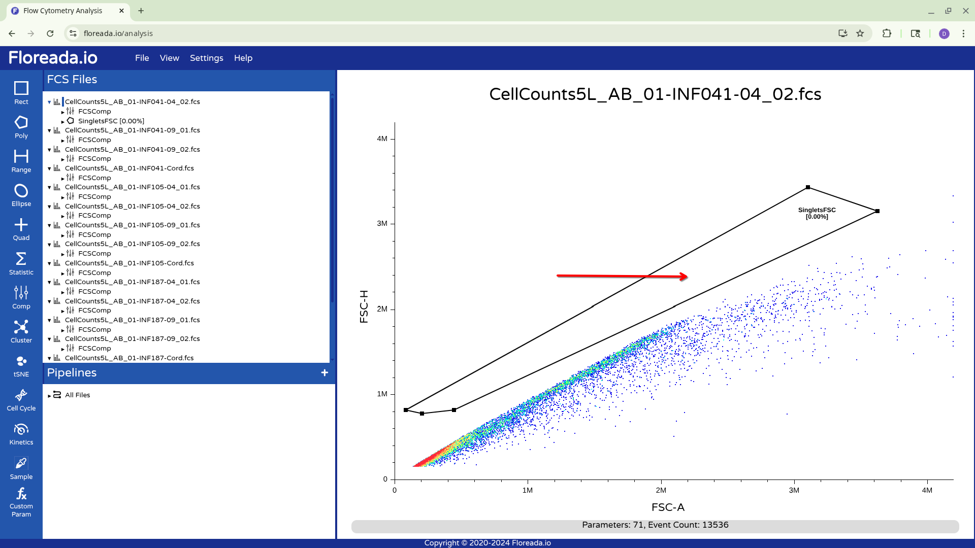
To move the entire gate, first click on a node to select the gate, then click in the center of the gate to adjust its location.
Additional Gates
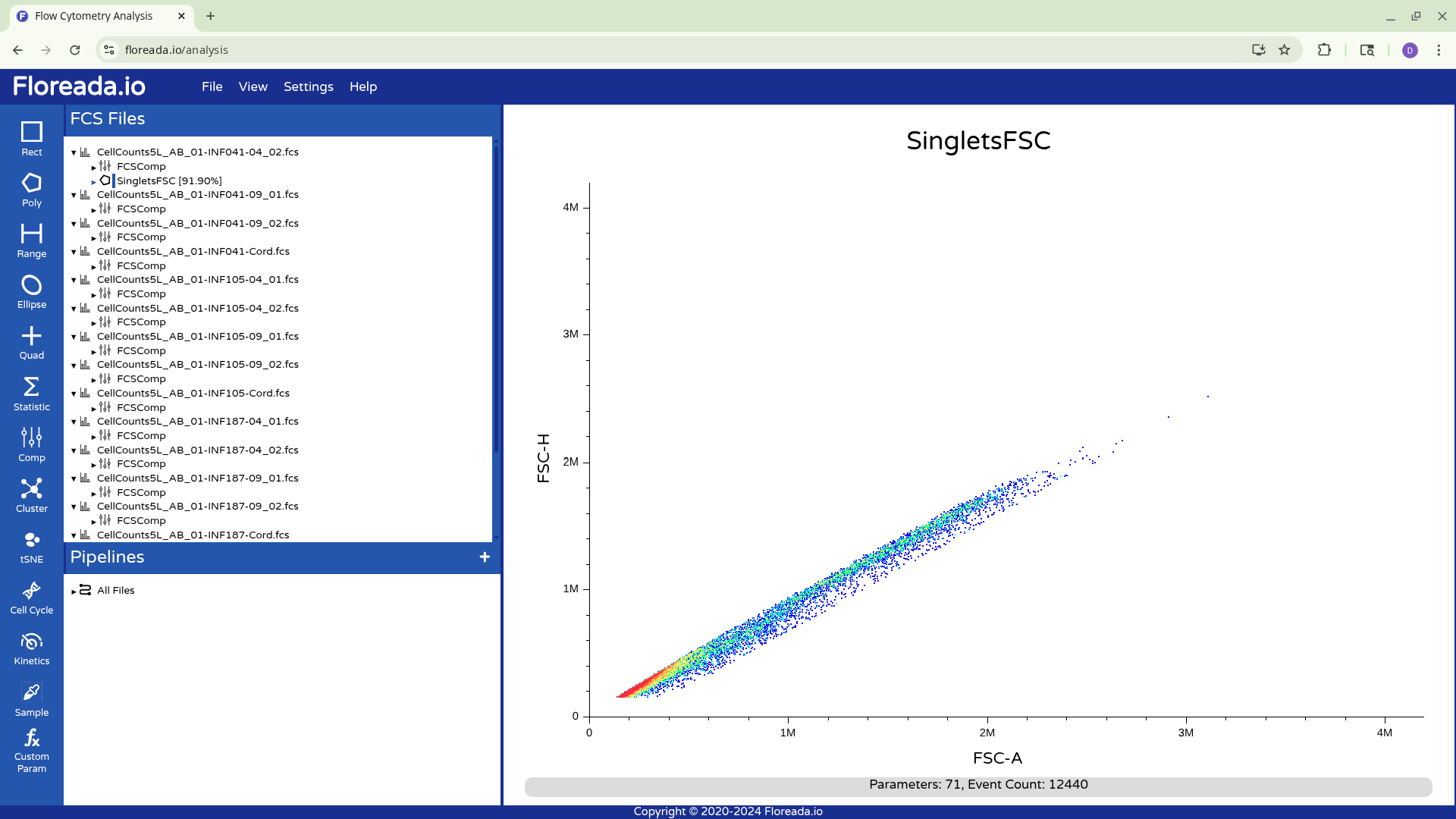
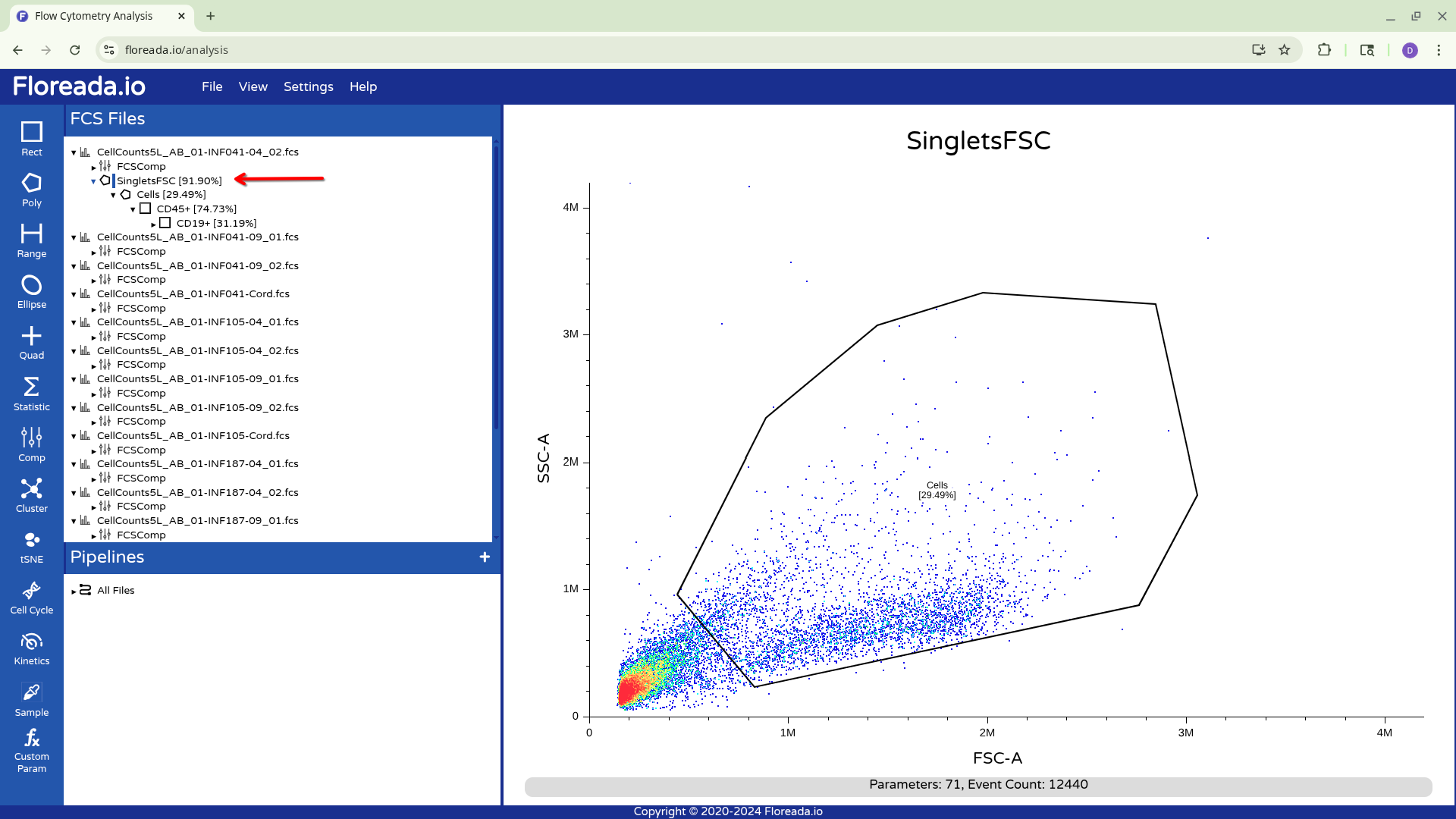
Unfortunately for those with the force-of-habit from using other softwares, double-clicking within the gate doesn’t do anything. To continue gating on the selected cells, you will need to click on the newly created gate name on the left. This will result in visualizing the isolated cells.
Once this is done, you can repeat the previous steps to change the axis markers and create a second gate. For this example, we went with a “Cells” gate to exclude debris from this particular sample.
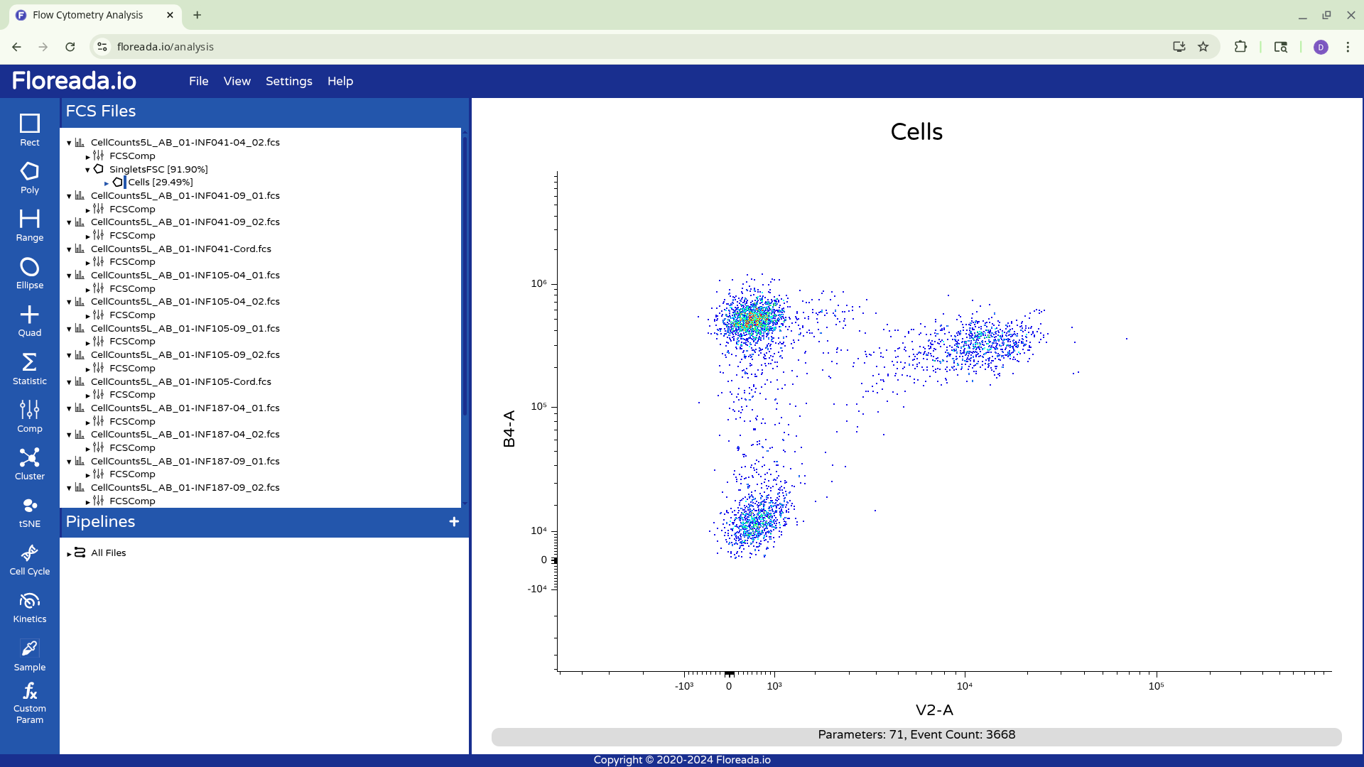
Having created the “Cells” gate, we will be switching gating based on FSC and SSC to using the detector parameters.
The samples in this example were acquired to derive the cell counts and concentration of various cell populations within cryopreserved cord and peripheral blood mononuclear cells (CBMC and PBMC) specimens after thawing.
They were stained with CD19 BV421, CD45 PE, and CD14 APC on a 5-Laser Cytek Aurora, before unmixing, this would correspond respectively to V1, YG1/B4, R1/YG4 peaks respectively.
Scaling/Transformation
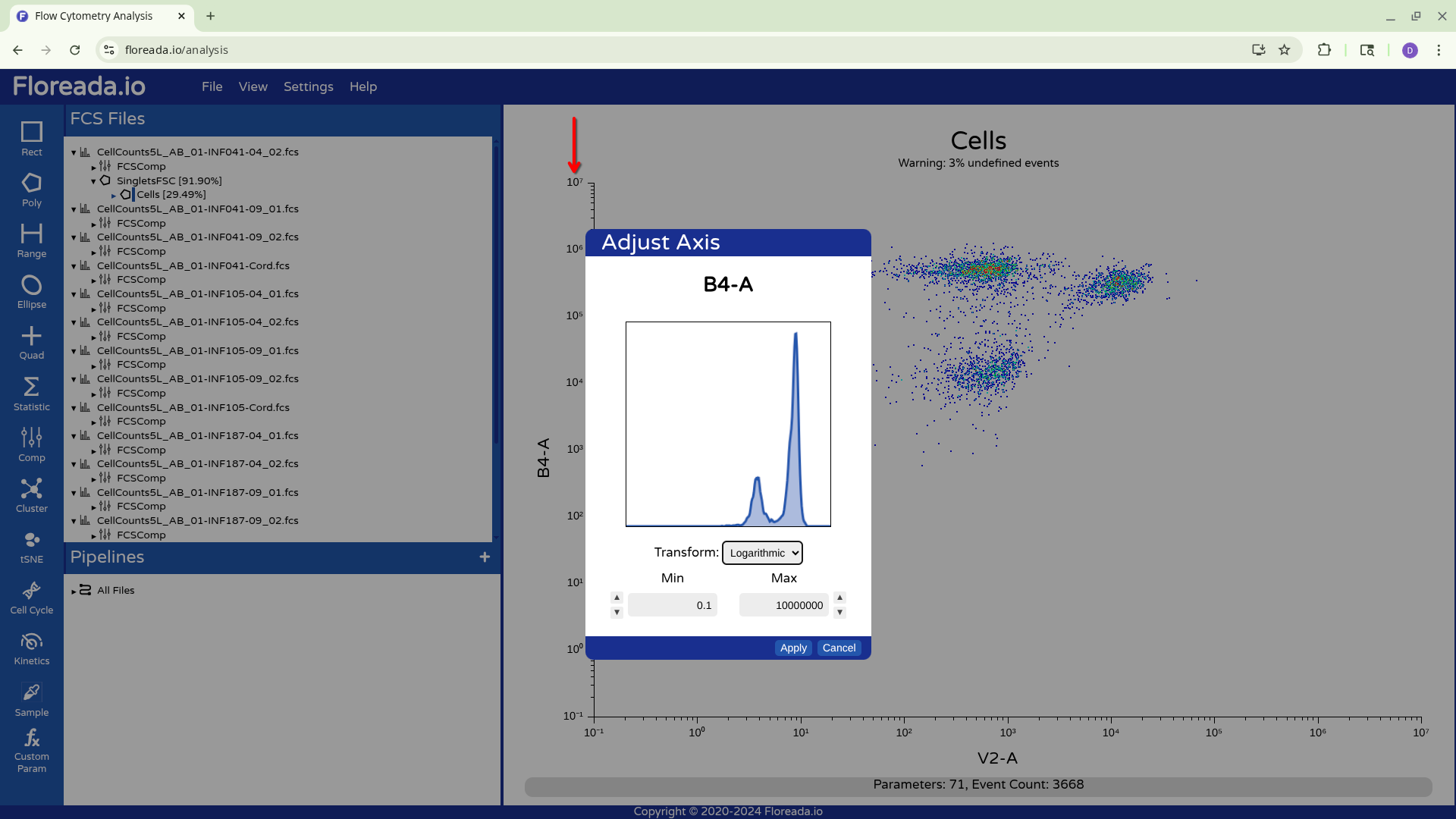
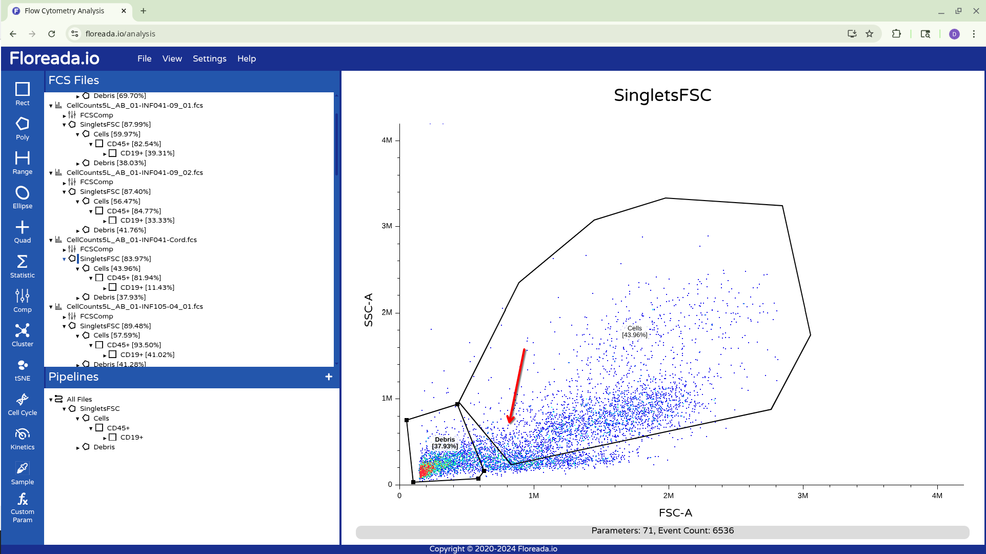
When we switch the axis, we can see that the scaling/transformation is not ideal, as the staining and not-staining populations are scrunched up together in the center of the plot.
![]()
To change the scaling/transformation, we need to click directly on the axis.
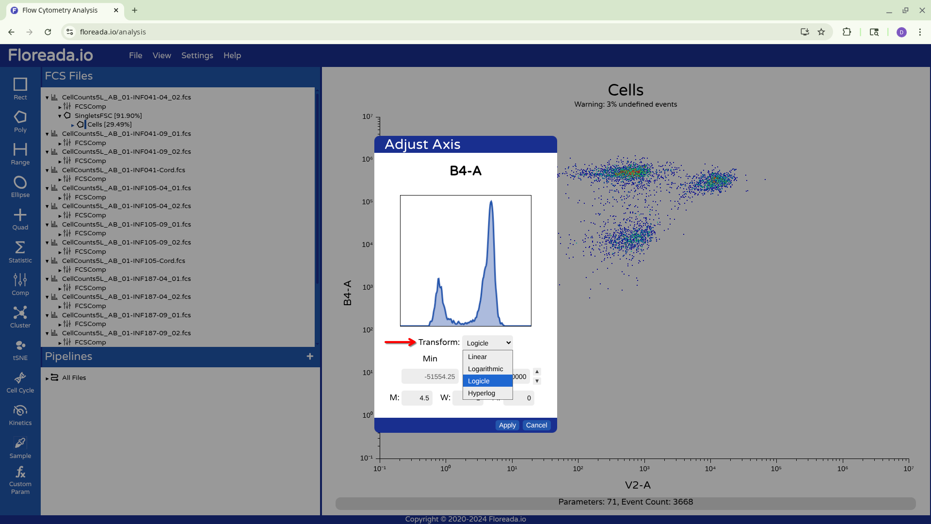
From there, when we click on the drop-down, we see the various transformation options. We will select Logicle, given we are working with spectral flow cytometry files.
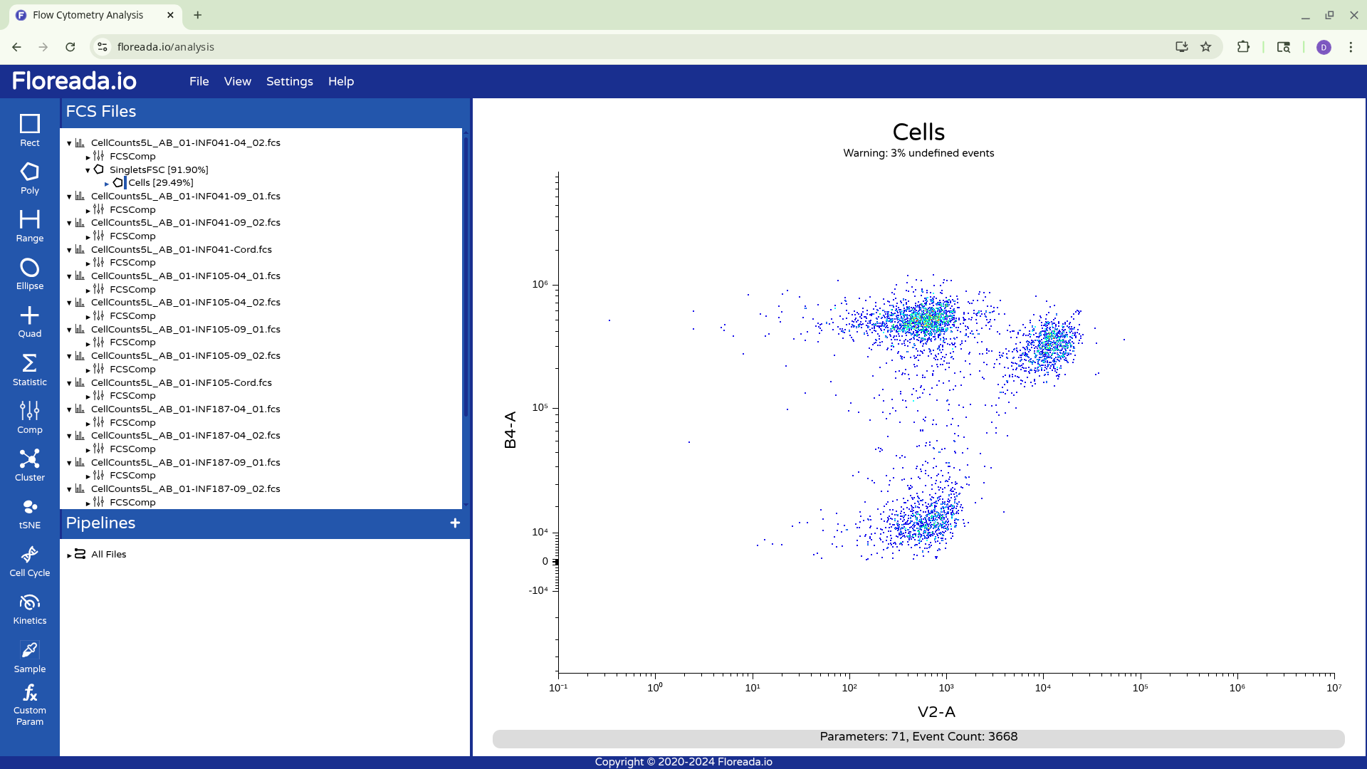
This y-axis values are subsequently visualized with the logicle transformation applied, increasing our resolution between the positive and negative population.
We can then repeat this for the x-axis, adjusting the fine-tune options for the scaling as needed.
Navigating Gating Hierarchy
With this done, let’s first draw a rectangle gate for the CD45+ (B4-A) cells.

And then selecting that population by clicking on the gate name, let’s proceed and gate the CD19+ cells (V2-A).
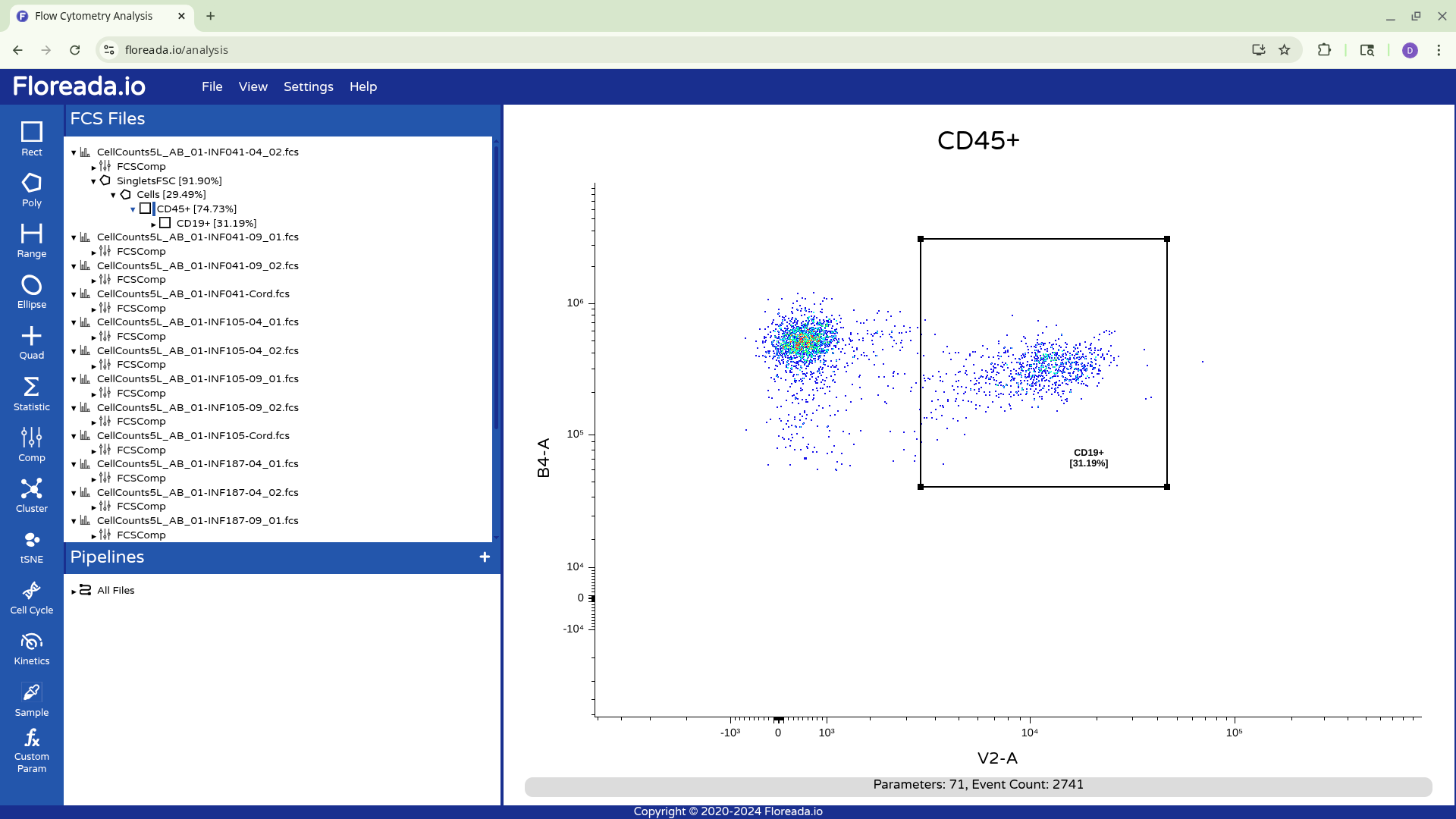
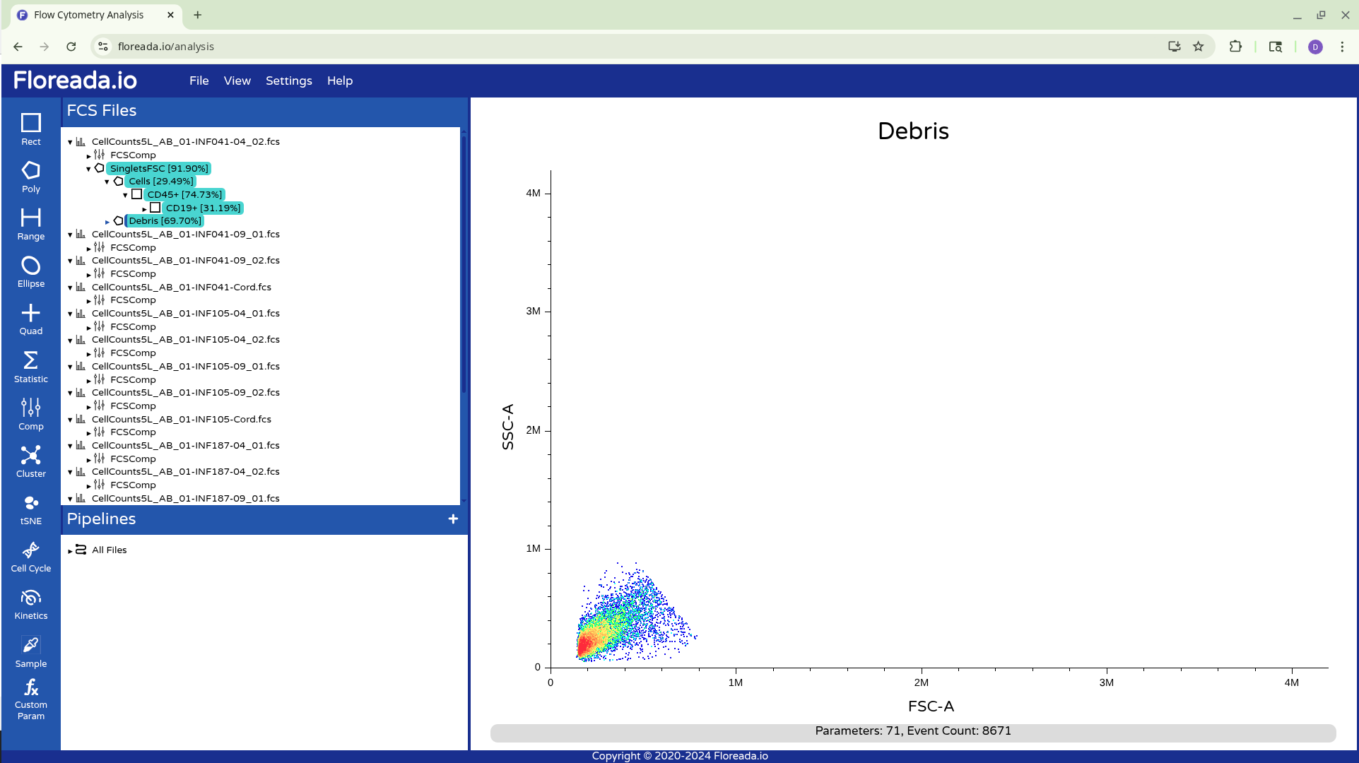
As you can see, we now have the various gates present in the gating hierarchy for the respective .fcs file. To return to a previous gated population, we would click on the parent population above it.
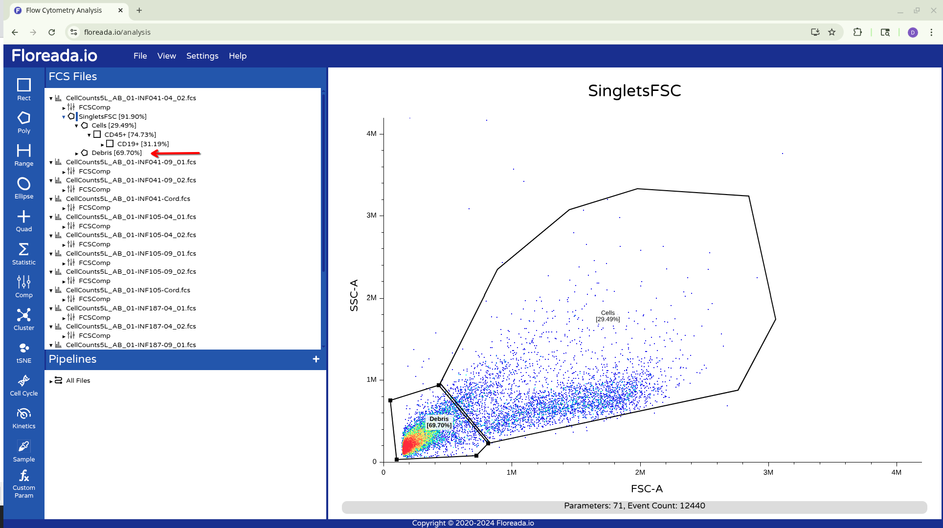
We can subsequently add an additional gate at this gating level for the likely debris population (the threshold setting was suboptimal for this experimental run).
Copying Gates
This was the process for gating for a single specimen. To copy gates over to the other specimens, we have two options. First, holding down your Ctrl (or equivalent) button, you can click on the individual gate names.
From there, you can drag them down to the next specimen and apply them.

Alternatively, you can drag down the highlighted gated to the Pipelines Tab, and apply to All Files. This will result in the gates being copied to all specimens in the experiment.
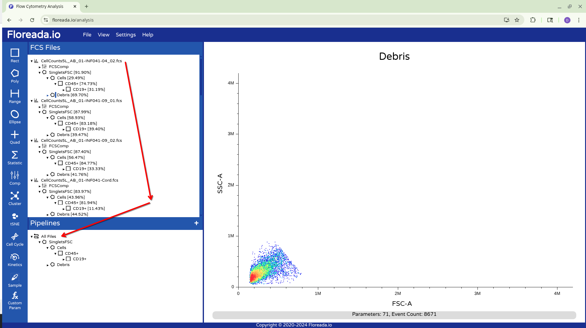
Adjustments within Pipelines will carry over to all other respective unmodified specimens that share it’s gates.
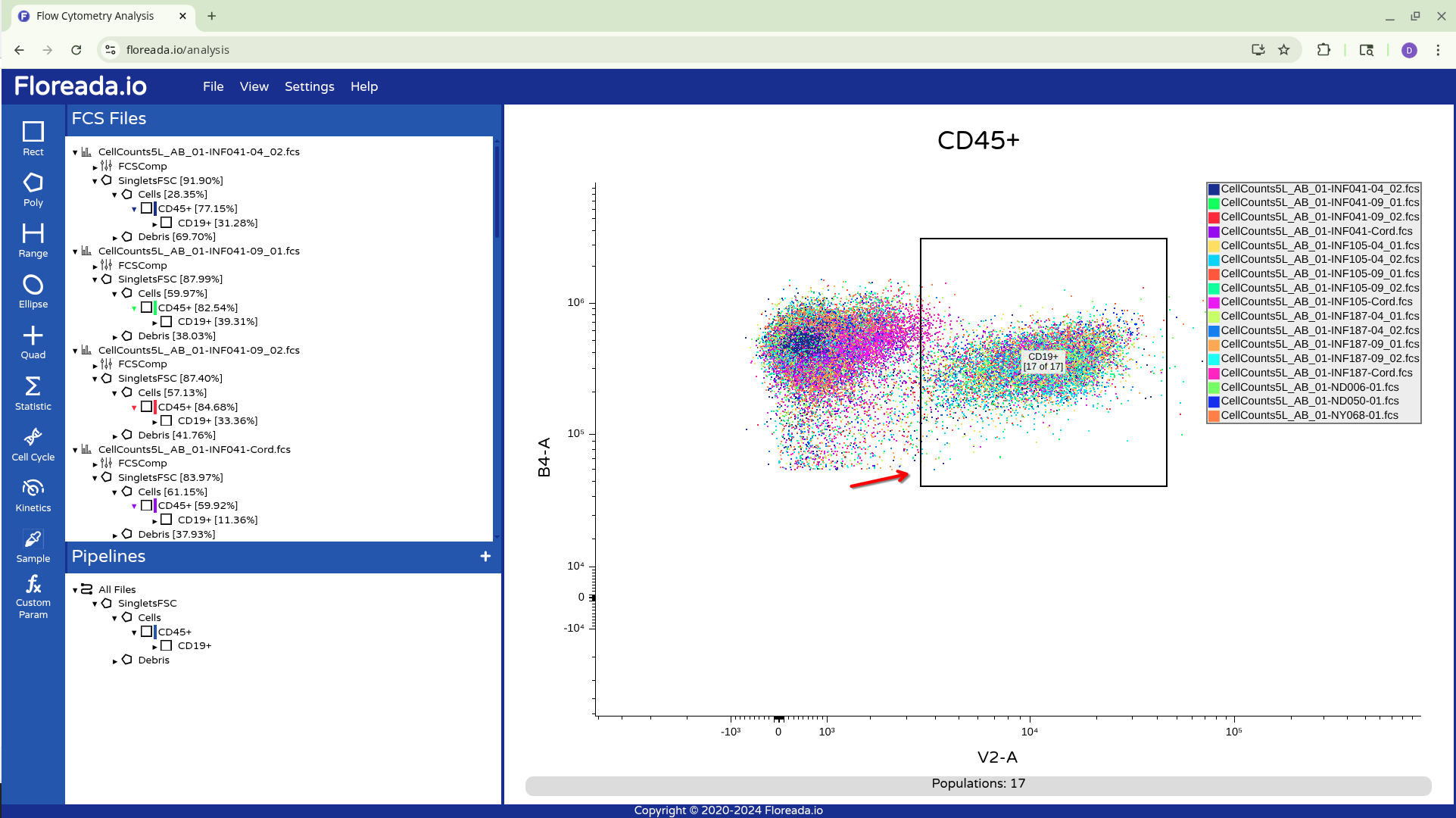
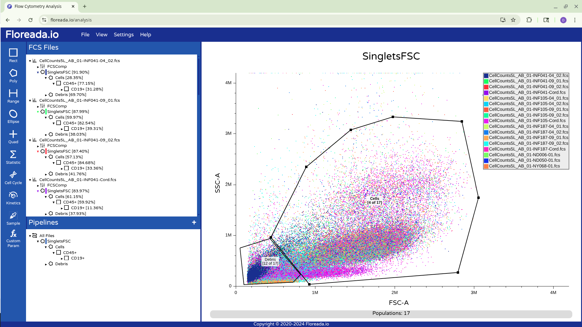
Once this is done, I recommend cycling through the gates for each specimen, just to ensure that the gates were positioned correctly before saving the workspace.
Saving Workspace
With everyone now “correctly” gated, we can proceed to save the workspace so that we can reopen it later from another browser.
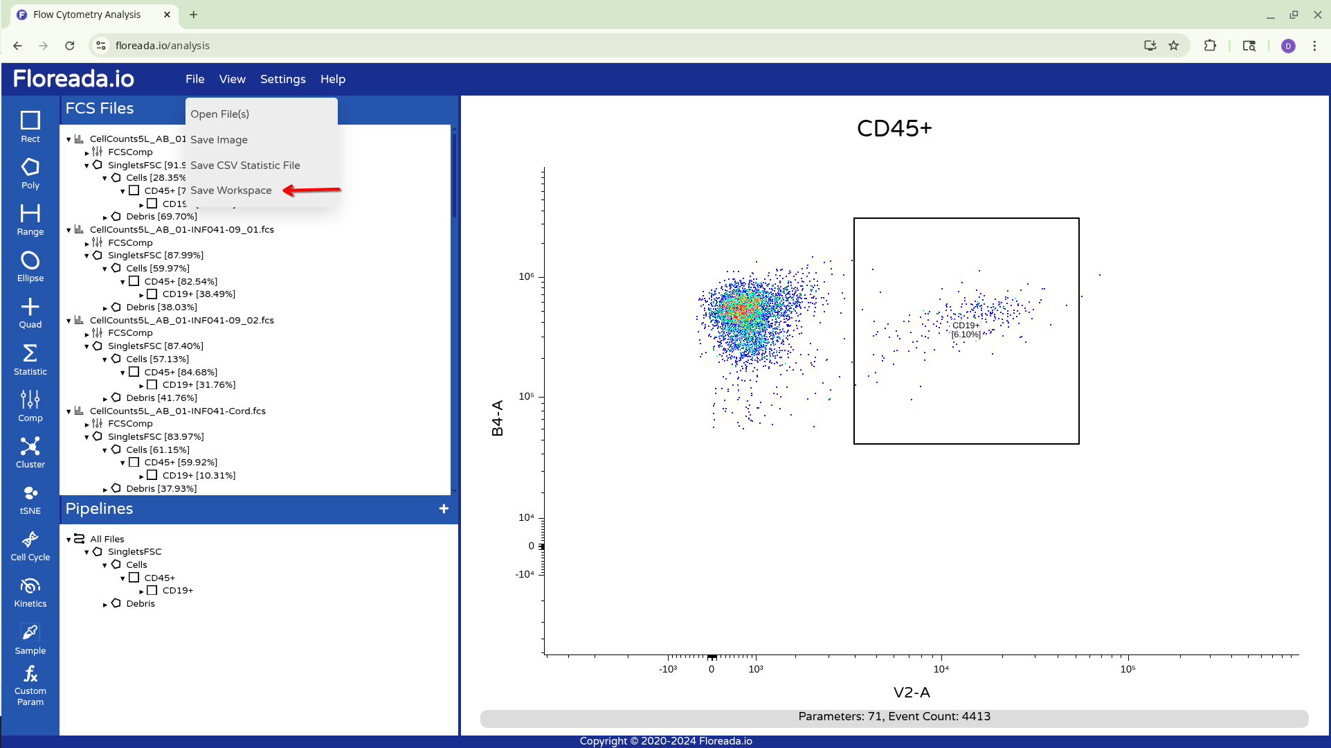
To do this we open the File tab from the upper navigation bar, and select Save Workspace.
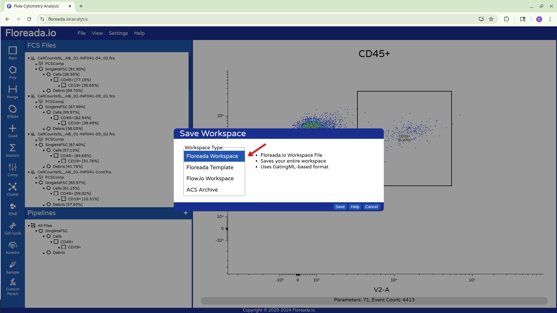
From there we have a couple options, for now let’s select Floreada Workspace. Where it is saved at will depend on your individual browser settings, so watch for a popup.
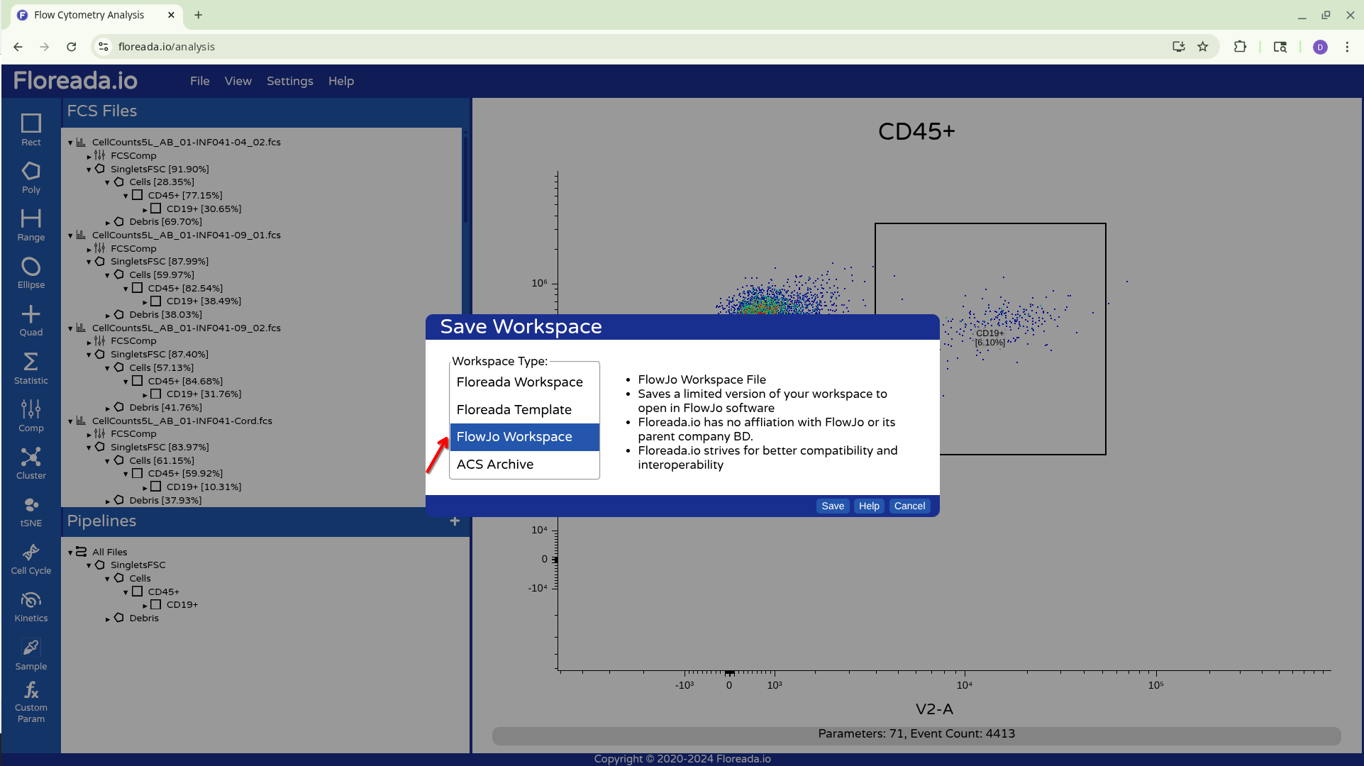
Alternatively (and crucially for the CytoML pipeline) we can also choose to save it as a FlowJo v10 .wsp file.
In both cases, you will end up with Workspace files that can be used later to access your created gates
Reopening Workspace
To reopen the Floreada workspace within the browser, reopen the website, and select the Open File(s) option.
From there, select both the Floreada Workspace file as well as the .fcs files
At which point you will now be back to the point you last saved at.
CytoML
Due to a unknown formatting bug, the Floreada produced FlowJo v10 .wsp is not directly accessible by CytoML at the time of this course. However, the issue is resolved as soon as the file is opened the first time within FlowJo v10, regardless of whether you have a log in or not. Strange? Yes, but we will take the workaround.
So, for anyone on Windows or MacOS, download FlowJo v10. Once installed, open the software, and close the login popups. Once there, open the Floreada created FlowJo.wsp file. Since you haven’t logged in, it won’t show any events. But it will correct the formatting bug. Close the software, and return to R. Your Floreada sourced .WSP file should now be readable by CytoML.
Odd? For sure. Fixable? Likely, I will set a reminder to work with the Floreada and CytoML devs to see if we can cut out the need for this workaround.
Wrap-up
Additional Resources