01 - Installing R Packages

Author

David Rach

Published

February 1, 2026

For screen-shot slides, click here

For the YouTube livestream recording (starting Wednesday), click here

Welcome to the first week of Cytometry in R! This week we will be diving into how R packages work, and the how to go about installing them.

Before getting started, please make sure you have completed the creating a GitHub and Workstation Setup walk-throughs, since we will begin where they left off once the required software was successfully installed.

Important

Please make sure to sync your forked version of the CytometryInR repository, and pull any changes to your local computer’s CytometryInR project folder so that you have the most recent version of the code and data available.

Background

During Workstation Setup, you installed the R software to your local computer. R as a programming language that started up in the 1990s. While its original focus was on statistics, it is now widely used in various fields thanks to contributions of many open-source developers over the years.

This expanded reach is in part due to the ability to create R packages, that encapsulate additional functions, that can do new things beyond what the original software (ie. base R) was capable of doing.

Currently, there are thousands of R packages available. Furthermore, there is a vibrant community of individuals that help maintain and document how to use these packages, which has helped sustain and grow the R ecosystem over the last couple decades.

Regardless if you are working with flow cytometry, or in ecology, or in econometrics, or political science, a lot of the analysis and visualizations that you see in publications often involve R.

Tip

R packages can also just be made for fun! Among my favorite examples of this, there is an R package that lets you add the snake game to your recalculating screen, as well as R packages that provide the color-palette schemes needed to make your plots with Studio Ghibli, Wes Anderson, or Bluey colors.

These R packages start off as source code (which is what we will be learning to write during this course). When you install a R package to your computer, this human-readable source code gets converted into a binary format with which your computer can interact directly.

Expanding on this concept, a new R package can be made up of new code (primarily in the form of tools (ie. functions) that do a particular useful things) that is entirely self-contained, or reuse functions present in existing R packages to help make something new. When an R package relies on a function from another R package, it needs the other R package to be installed in order for everything to work properly. This is known as a package dependency.

To make distributing the thousands of R packages and their associated package dependencies easier, R packages are collected (ie. hosted) within repositories, which function as an intermediate distributor.

The three main locations for R packages from are CRAN (containing 23069 packages), Bioconductor (containing 2361 packages), and individual R packages hosted by their developers via GitHub.

The process of installing R packages will vary a bit depending on which repository the respective R package is in. For beginners, this often prooves to be a pain-point, as they will attempt to install an R package using one set of installation commands, only to get an error (because the R package is not in that repository).

In this session, we will work on installing the various R packages we will need through the course. While doing so, we will explore how to figure out which repository the individual package is in; what installation commands to use to download it; and how to look up the help documentation. We will also touch on how the functions within an R package are made available for our computer to use (via the library() call), and how to troubleshoot the more commonly encountered installation errors.

Getting Started

Set Up

Alright, with the background out of the way, let’s get started!

Important

Warning

Please remember to always copy over the new material from your local CytometryInR folder to a separate Project Folder that you created and named (ex. “Week_01” or “MyLearningFolder”, etc.). This will ensure any edits you make to the files do not affect your ability to bring in next week’s materials to the CytometryInR folder

After pulling the new data and code locally, open CytometryInR, open the course folder, and open the 01_InstallingRPackages folder. From here, copy the index.qmd file to your own working Project Folder (ex. Week_01) where you can work on it without causing any conflicts. Then return to Positron and open up your working project folder (ex. Week_01).

Next up, within Positron, let’s make sure to select R as the coding language being used for this session.

Now that R is running within Positron, the console (lower portion of the screenn) is now able to run (ie. execute) any R code that is sent to it.

Checking for Loaded Packages

For the contents (ie. the functions) of an R package to be available for your computer to use, they must first be activated (ie. loaded) into your local environment. We will first learn how to check what R packages are currently active.

Accessing Help Documentation

Within your own index.qmd (or a new .qmd file that you created), type out/copy-paste the following sessionInfo() function:

sessionInfo()

If you hover over the line of code within Positron, you will glimpse the help file for the particular function you are hovering over.

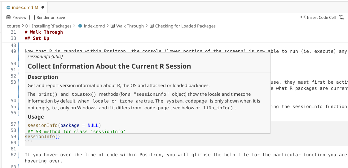
In this case, we can see the help documentation corresponding for sessionInfo(). Beyond hovering over the function, this can also be accessed by adding a ? directly in front of the function, and then running that line of code.

?sessionInfo()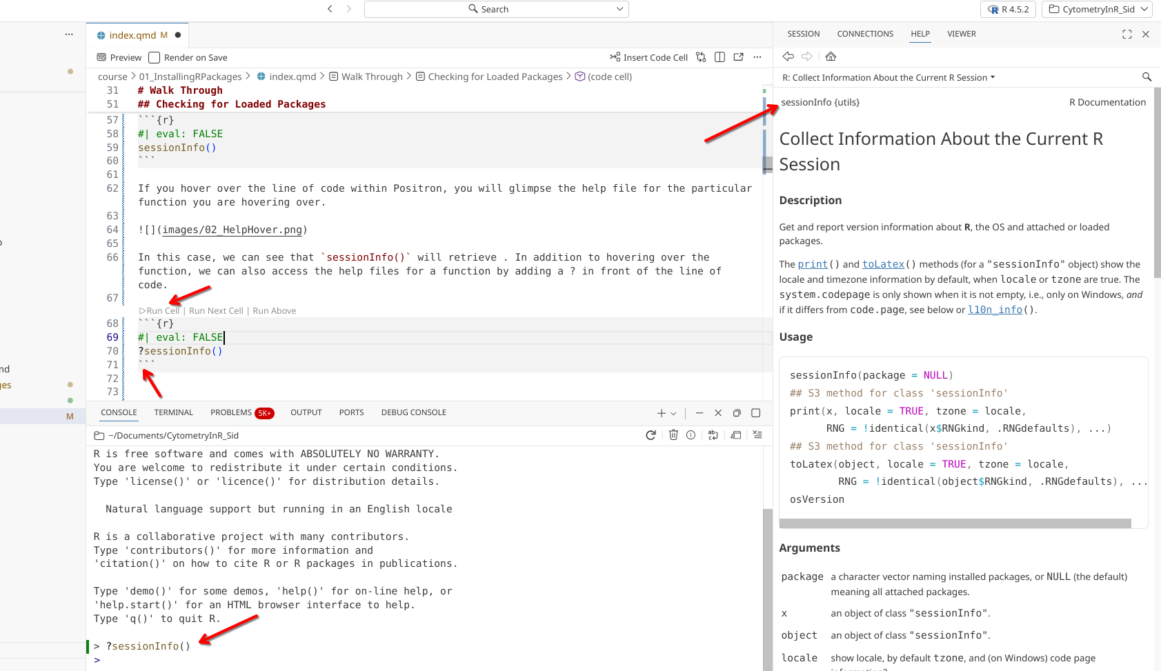

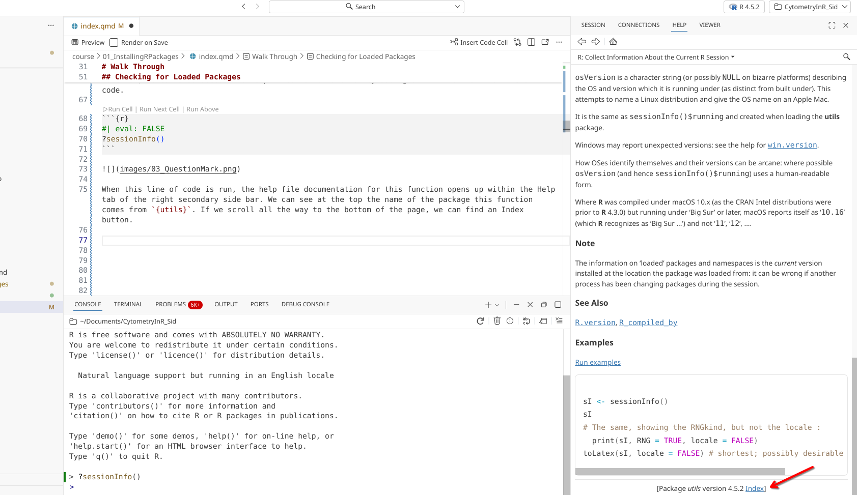
When executed, the function’s help file documentation will open up within the Help tab in the secondary side bar on the right-side of the screen. Glancing at the top of the page we can see the name of the package that contains the sessionInfo() function ({utils}). Scrolling down the help page past all the documentation, we can see a link to the index page.

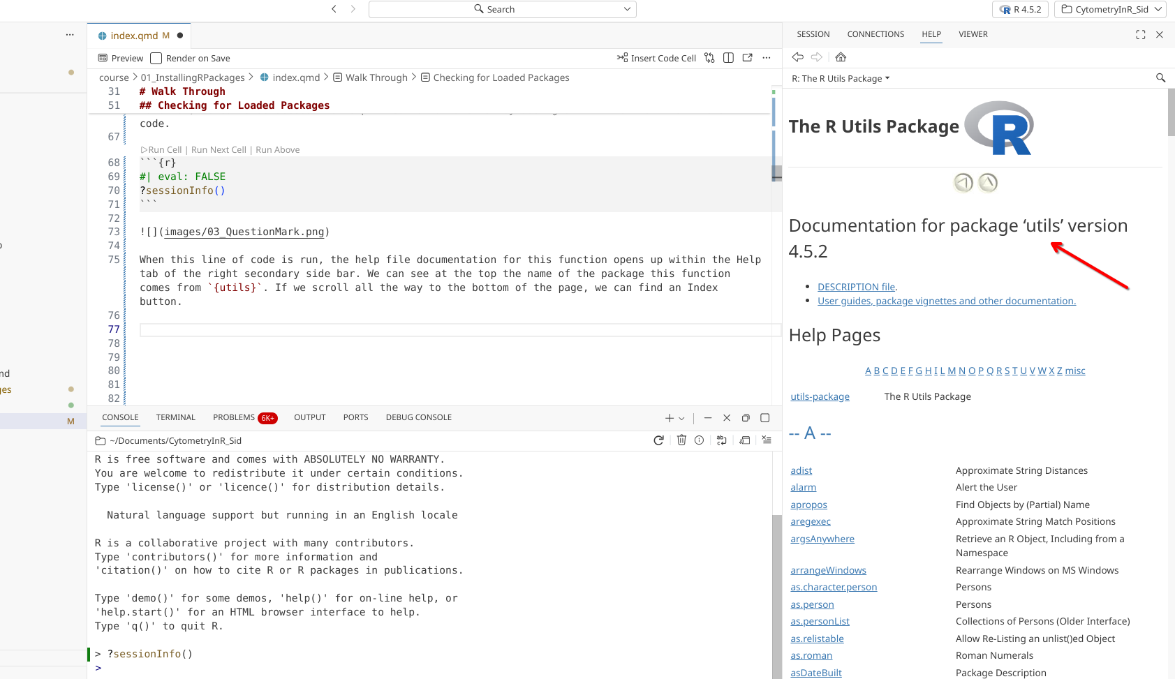
After clicking, the Help tab switches from viewing the documentation for the sessionInfo() function, to showing all the functions within the utils package. Most R packages contain help documentation, so this process can be adapted to find out additional information about what a function does, and what arguments are needed to produce customized outputs.

sessionInfo()

Within your .qmd file, let’s go ahead and run the following code-block:

sessionInfo()

R version 4.5.2 (2025-10-31)
Platform: x86_64-pc-linux-gnu
Running under: Debian GNU/Linux 13 (trixie)

Matrix products: default
BLAS:   /usr/lib/x86_64-linux-gnu/blas/libblas.so.3.12.1 
LAPACK: /usr/lib/x86_64-linux-gnu/lapack/liblapack.so.3.12.1;  LAPACK version 3.12.0

locale:
 [1] LC_CTYPE=en_US.UTF-8       LC_NUMERIC=C              
 [3] LC_TIME=en_US.UTF-8        LC_COLLATE=en_US.UTF-8    
 [5] LC_MONETARY=en_US.UTF-8    LC_MESSAGES=en_US.UTF-8   
 [7] LC_PAPER=en_US.UTF-8       LC_NAME=C                 
 [9] LC_ADDRESS=C               LC_TELEPHONE=C            
[11] LC_MEASUREMENT=en_US.UTF-8 LC_IDENTIFICATION=C       

time zone: America/New_York
tzcode source: system (glibc)

attached base packages:
[1] stats     graphics  grDevices utils     datasets  methods   base     

other attached packages:
[1] BiocStyle_2.38.0

loaded via a namespace (and not attached):
 [1] htmlwidgets_1.6.4   BiocManager_1.30.27 compiler_4.5.2     
 [4] fastmap_1.2.0       cli_3.6.5           tools_4.5.2        
 [7] htmltools_0.5.9     otel_0.2.0          yaml_2.3.12        
[10] rmarkdown_2.30      knitr_1.51          jsonlite_2.0.0     
[13] xfun_0.56           digest_0.6.39       rlang_1.1.7        
[16] evaluate_1.0.5

The outputs that get returned by sessionInfo() will vary a bit depending on your computer’s operating system, and the version of R you have installed.

For today, let’s focus on the last two elements of the output:

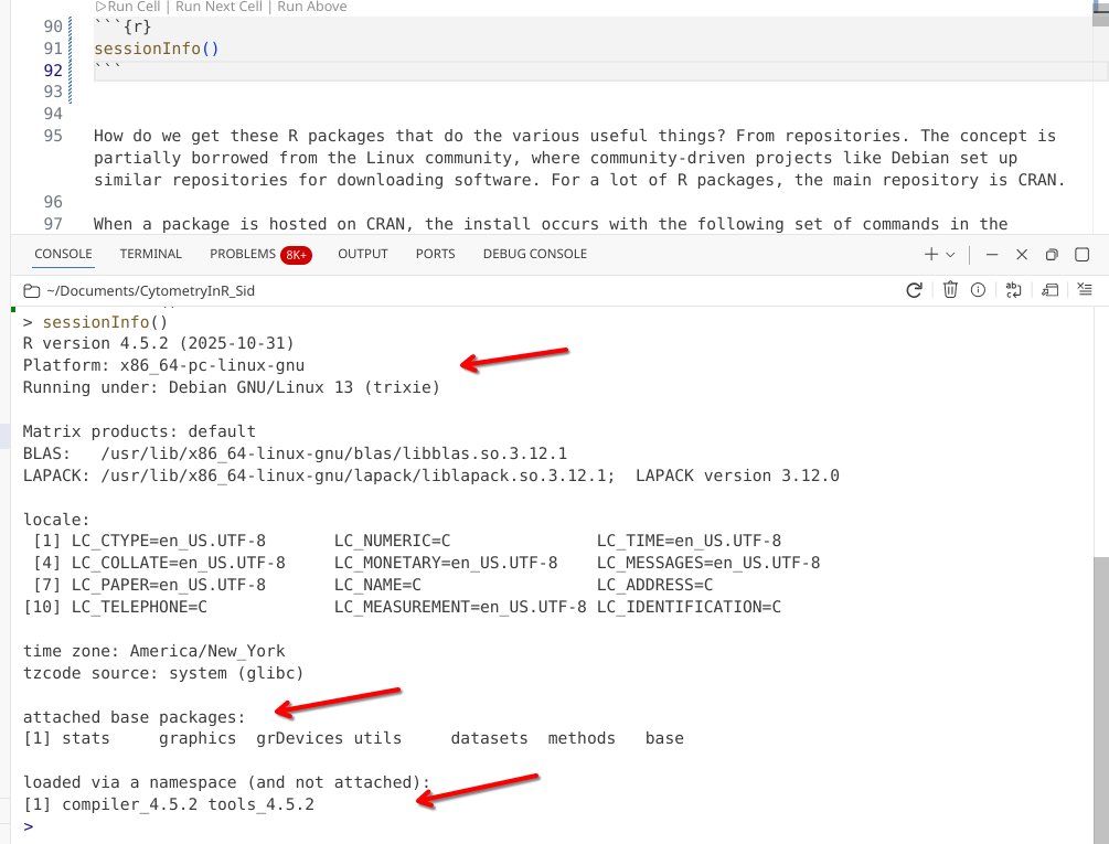
The R software itself is made up of several base R packages, that are loaded automatically. These contain everything you need to read, write and run R code on your computer. You can see these packages are the stats, graphics, grDevices, utils, datasets, methods and base packages.

As we install additional R packages and load them using the library() function throughout this session, sporadically re-run sessionInfo() to see how this list of R packages changes.

Installing from CRAN

We will start by installing R packages that are part of the CRAN repository. This is the main R package repository, being part of the broader R software project. In the context of this course, R packages that work primarily with general data structure (rows, columns, matrices, etc.) or visualizations will predominantly be found within this repository.

These include the tidyverse packages. These packages have collectively made R easier to use by smoothing out some of the rough edges of base R, which is why R has seen major growth within the last decade. We will be installing several of these R packages today.

dplyr

Our first R package we will install during this session is the dplyr package. Since it is hosted on the CRAN repository, to install it, we will need to use the CRAN-specific installation function install.packages().

?install.packages()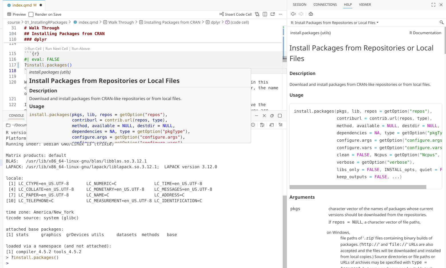

For the install.packages() function, we place within the () the name of the R package from CRAN that we wish to install.

install.packages("dplyr")

Tip

A usual struggle point for beginners is that install.packages() requires ” ” to be placed around the package name. Forgetting them results in the error that we see below.

install.packages(dplyr)

Error:
! object 'dplyr' not found

install.packages("dplyr")

Go ahead and click on “Run Cell” next to your code-block, to install the dplyr R package.

When a package starts to install, you will see your console start to display text resembling that seen in the image below (varying a bit depending on your computers operating system).

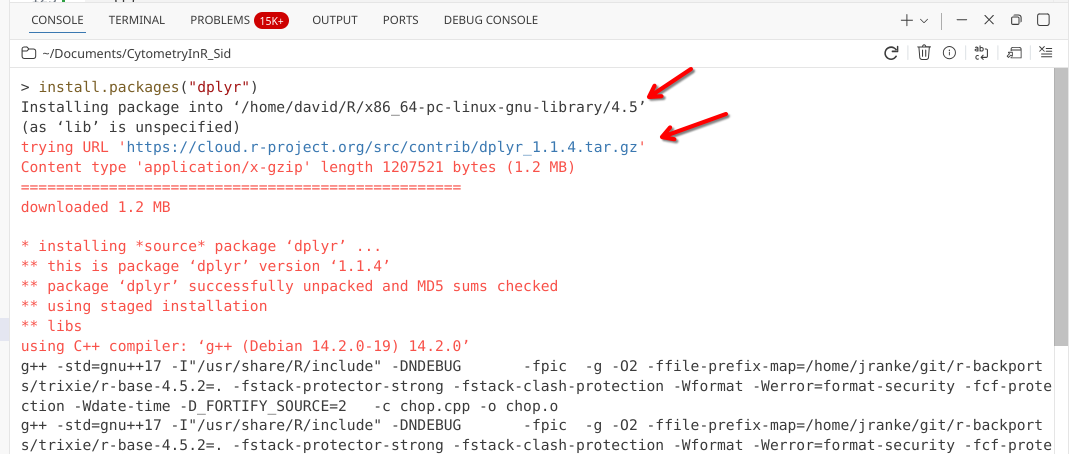
Within this opening scrawl, you will see the location on your computer the R package is being installed to, as well as the file location for the R package being retrieved on CRAN.

If the package is successfully located, your computer will proceed to first download, then unpack (ie. unzip) it, before attempting to install to the target folder.

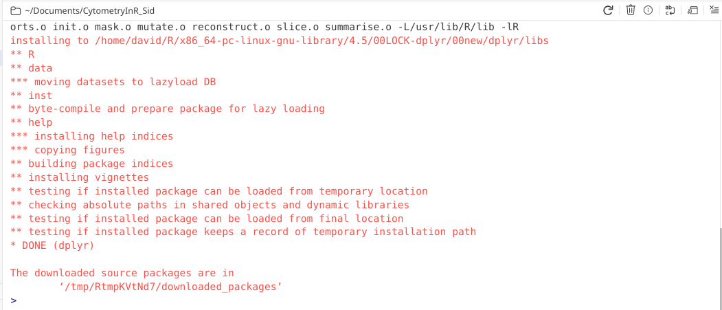
The final steps of the installation process involved various steps to verify everything was copied successfully, the help documentation assembled, and that the R package is capable of being loaded. If this is the case, you will see the “Done” line appear, as well as a mention where the original downloaded source package files has been stashed (usually a temp folder).

Attaching packages via library()

If an R package has been installed successfully, we are now able to load it (ie. make it’s functions available) to our local environment using the library() function.

?library()

Unlike install.packages(), where we needed “” around the package name, the library() function does not require “” around the package name. Let’s go ahead and load in dplyr, making its respective functions to our local environment.

library(dplyr)


Attaching package: 'dplyr'

The following objects are masked from 'package:stats':

    filter, lag

The following objects are masked from 'package:base':

    intersect, setdiff, setequal, union

From the output, we can see that dplyr has been attached. There are also a couple functions within dplyr that have identical names to functions within the stats and base packages. To avoid confusion, these 6 functions are masked, which is why we get the additional messages.

With dplyr now loaded via the library() call, let’s check sessionInfo() to see what has changed.

sessionInfo()

R version 4.5.2 (2025-10-31)
Platform: x86_64-pc-linux-gnu
Running under: Debian GNU/Linux 13 (trixie)

Matrix products: default
BLAS:   /usr/lib/x86_64-linux-gnu/blas/libblas.so.3.12.1 
LAPACK: /usr/lib/x86_64-linux-gnu/lapack/liblapack.so.3.12.1;  LAPACK version 3.12.0

locale:
 [1] LC_CTYPE=en_US.UTF-8       LC_NUMERIC=C              
 [3] LC_TIME=en_US.UTF-8        LC_COLLATE=en_US.UTF-8    
 [5] LC_MONETARY=en_US.UTF-8    LC_MESSAGES=en_US.UTF-8   
 [7] LC_PAPER=en_US.UTF-8       LC_NAME=C                 
 [9] LC_ADDRESS=C               LC_TELEPHONE=C            
[11] LC_MEASUREMENT=en_US.UTF-8 LC_IDENTIFICATION=C       

time zone: America/New_York
tzcode source: system (glibc)

attached base packages:
[1] stats     graphics  grDevices utils     datasets  methods   base     

other attached packages:
[1] dplyr_1.1.4      BiocStyle_2.38.0

loaded via a namespace (and not attached):
 [1] digest_0.6.39       R6_2.6.1            fastmap_1.2.0      
 [4] tidyselect_1.2.1    xfun_0.56           magrittr_2.0.4     
 [7] glue_1.8.0          tibble_3.3.1        knitr_1.51         
[10] pkgconfig_2.0.3     htmltools_0.5.9     generics_0.1.4     
[13] rmarkdown_2.30      lifecycle_1.0.5     cli_3.6.5          
[16] vctrs_0.7.1         compiler_4.5.2      tools_4.5.2        
[19] evaluate_1.0.5      pillar_1.11.1       yaml_2.3.12        
[22] otel_0.2.0          BiocManager_1.30.27 rlang_1.1.7        
[25] jsonlite_2.0.0      htmlwidgets_1.6.4

Similar to what was seen for the base R packages, dplyr is now attached. This means we should theoretically now have access to all its functions. We can verify this by seeing if we can look up the dplyr packages select() function and it’s respective help page.

?select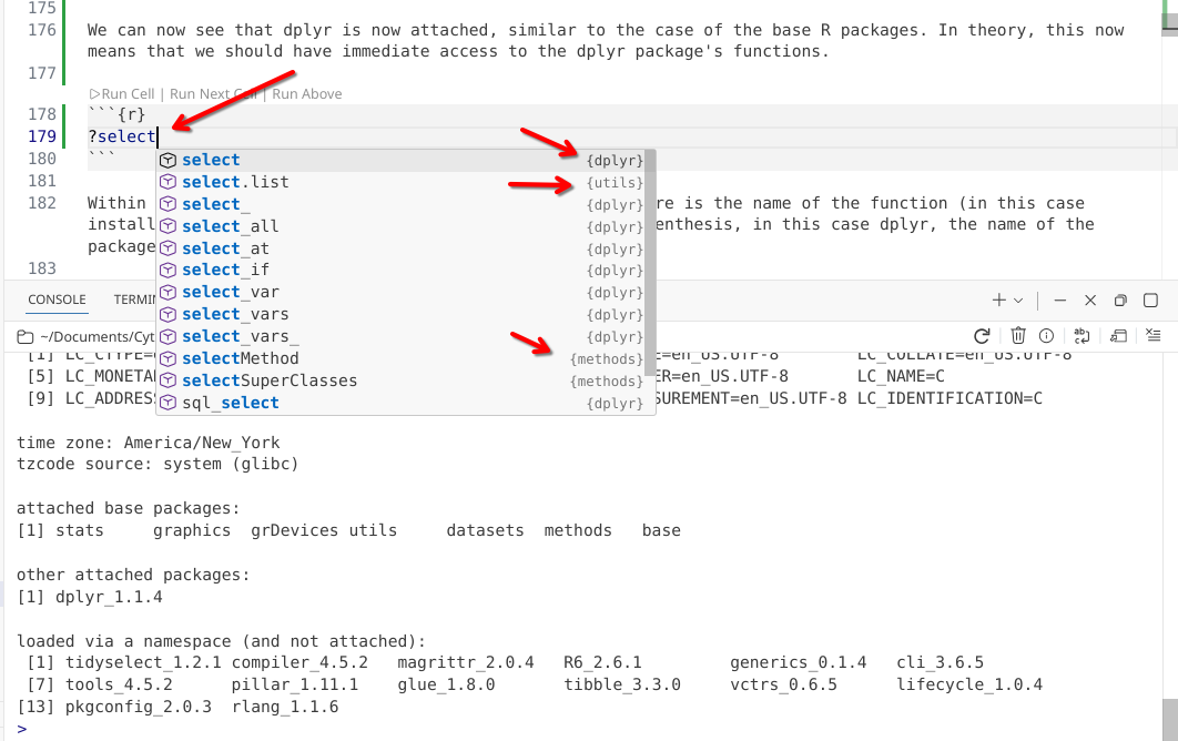

Since its parent package has been attached to our local environment (via the library() call), we can see dplyr functions appear as suggestions as we begin to type.

By contrast, is we check for the ggplot() function from the ggplot2 package (which we haven’t yet installed or attached via library()), no suggestions will pop up.

?ggplot

No documentation for 'ggplot' in specified packages and libraries:
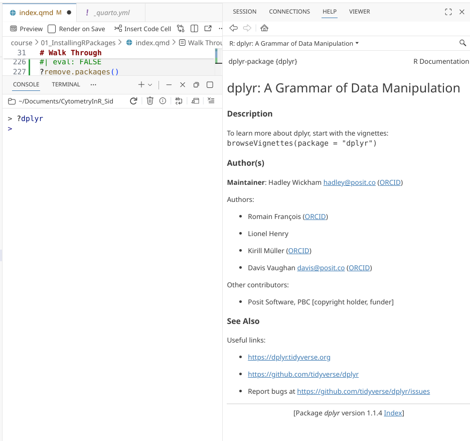
you could try '??ggplot'

Beyond individual functions, some R packages also have help landing pages, that can be similarly accessed by adding a ? in front of the package name:

Unattaching

So far, we have installed an R package, and then attached it (via library()). How would we reverse these steps?

Well, to unload it from the local environment, there are a couple options. You could of course simply shut down Positron. The local environment only exist in context of when you open and close the session, which closing the program will do. All previously loaded R packages will be unattached, which is why when you start a new session you will need to load in all packages you plan on using via library().

Alternatively, although less used, you could detach() it via your console:

detach("package:dplyr", unload=TRUE)

sessionInfo()

R version 4.5.2 (2025-10-31)
Platform: x86_64-pc-linux-gnu
Running under: Debian GNU/Linux 13 (trixie)

Matrix products: default
BLAS:   /usr/lib/x86_64-linux-gnu/blas/libblas.so.3.12.1 
LAPACK: /usr/lib/x86_64-linux-gnu/lapack/liblapack.so.3.12.1;  LAPACK version 3.12.0

locale:
 [1] LC_CTYPE=en_US.UTF-8       LC_NUMERIC=C              
 [3] LC_TIME=en_US.UTF-8        LC_COLLATE=en_US.UTF-8    
 [5] LC_MONETARY=en_US.UTF-8    LC_MESSAGES=en_US.UTF-8   
 [7] LC_PAPER=en_US.UTF-8       LC_NAME=C                 
 [9] LC_ADDRESS=C               LC_TELEPHONE=C            
[11] LC_MEASUREMENT=en_US.UTF-8 LC_IDENTIFICATION=C       

time zone: America/New_York
tzcode source: system (glibc)

attached base packages:
[1] stats     graphics  grDevices utils     datasets  methods   base     

other attached packages:
[1] BiocStyle_2.38.0

loaded via a namespace (and not attached):
 [1] digest_0.6.39       R6_2.6.1            fastmap_1.2.0      
 [4] tidyselect_1.2.1    xfun_0.56           magrittr_2.0.4     
 [7] glue_1.8.0          tibble_3.3.1        knitr_1.51         
[10] pkgconfig_2.0.3     htmltools_0.5.9     generics_0.1.4     
[13] rmarkdown_2.30      lifecycle_1.0.5     cli_3.6.5          
[16] vctrs_0.7.1         compiler_4.5.2      tools_4.5.2        
[19] evaluate_1.0.5      pillar_1.11.1       yaml_2.3.12        
[22] otel_0.2.0          BiocManager_1.30.27 rlang_1.1.7        
[25] jsonlite_2.0.0      htmlwidgets_1.6.4

Looking at the sessionInfo() output, dplyr is no longer attached to the local environment. Consequently, if we try to once again look for the documentation, no information will be retrieved.

?dplyr

No documentation for 'dplyr' in specified packages and libraries:
you could try '??dplyr'

There is a workaround however, if we want to access functions from an unloaded R package. We can specify the R package’s name, followed by two :, and then the function name. The :: conveys the context to your computer that the package is present, but may not be attached.

?dplyr::select()

This particular use case can be useful if we want to run a particular function, but not load in all a packages functions (which may have identical function names to other R packages we are using and cause some conflicts).

Removing Packages

Just as we can install an R package, we can also uninstall an R package (although doing so is rare, most often when encountering package dependency conflict). To do so, we would use the remove.packages() function.

?remove.packages()

remove.packages("dplyr")

This results in the package being removed entirely from our computer. We would then need to reinstall it if needed in the future.

Common Issues

As previously mentioned, CRAN is the main repository for R packages. But what if we tried to install an R package that is only found on Bioconductor or via GitHub using the install.packages() function?

To see what occurs, let’s try installing the PeacoQC package (which is found on Bioconductor).

install.packages("PeacoQC")

Installing package into '/home/david/R/x86_64-pc-linux-gnu-library/4.5'
(as 'lib' is unspecified)

Warning: package 'PeacoQC' is not available for this version of R

A version of this package for your version of R might be available elsewhere,
see the ideas at
https://cran.r-project.org/doc/manuals/r-patched/R-admin.html#Installing-packages

As you can see, the initial warning message suggest that PeacoQC is not available for your version of R. When I first started trying to learn R on my own during COVID, this particular message was the bane of my existence and I couldn’t figure out what was going on.

This is just a default warning message, that would apply for both a package having a version mismatch, but also shown when trying to install packages that are not found on CRAN.

Installing from Bioconductor

Bioconductor is the second R package repository we will be working with throughout the course. While it contains far fewer packages than CRAN, it contains packages that are primarily used by the biomedical sciences. Following this link you can find it’s current flow and mass cytometry R packages.

Bioconductor R packages differ from CRAN R packages in a couple of ways. Bioconductor has different standards for acceptance than CRAN. They usually contain interoperable object-types, put more effort into documentation and continous testing to ensure that the R package remains functional across operating systems.

To install an R package that is located on Bioconductor, we first need to install the BiocManager package from CRAN. This package will allow us to install Bioconductor packages from their respective repository.

install.packages("BiocManager")

Once BiocManager is installed, we can attach it to our local environment using the library() function

library(BiocManager)

When loaded, you will see an output showing the current Bioconductor and R versions.

We can then use BiocManager’s install() function to go back and install PeacoQC().

Tip

As always, don’t forget the “” when running an install() command.

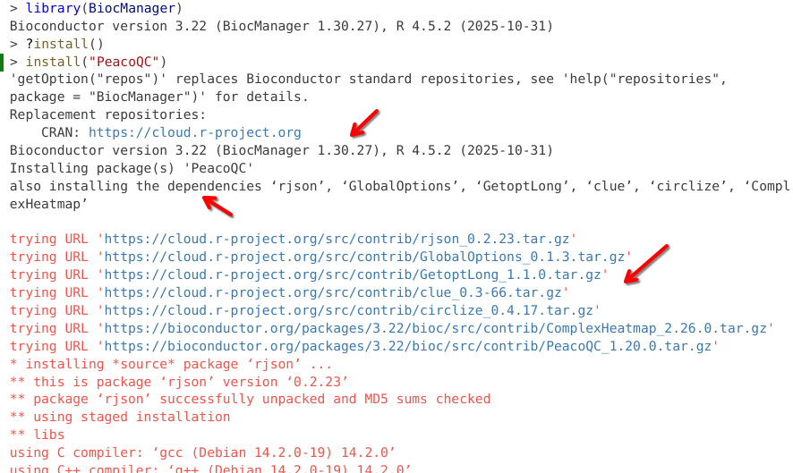
?install()

install("PeacoQC")

We see a similar opening sequence of installation steps as what we saw when installing the dplyr package from CRAN. However, in this case, several package dependencies (rjson, GlobalOptions, etc.) are present. Consequently, you can see these packages are also being downloaded from their respective repositories (either CRAN or Bioconductor), then unzipped and assembled before PeacoQC undergoes installation.

Note

Behind the scenes, within an R package, what package dependencies need to be installed are specified through the Description and Namespace files. If a package name is removed from these files, it will not be installed during the installation process

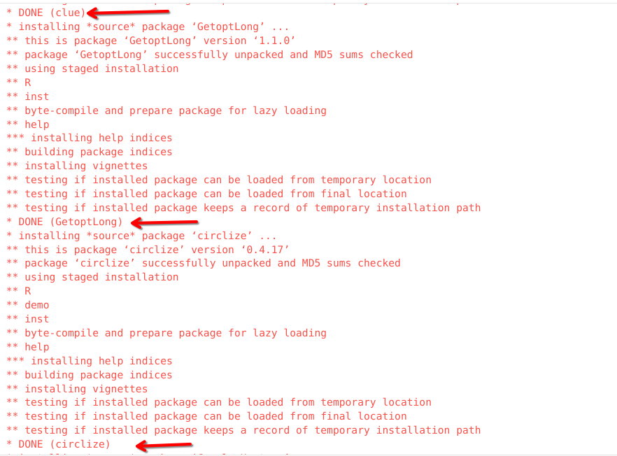
Within the scrawl of installation outputs, we can see individual dependencies undergoing installation similar to what we saw with dplyr, with a “Done (packagename)” being printed upon successful installation.

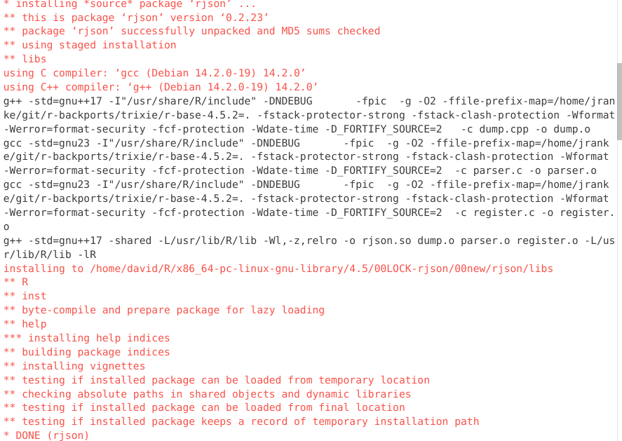
This process continues for each dependency being installed.

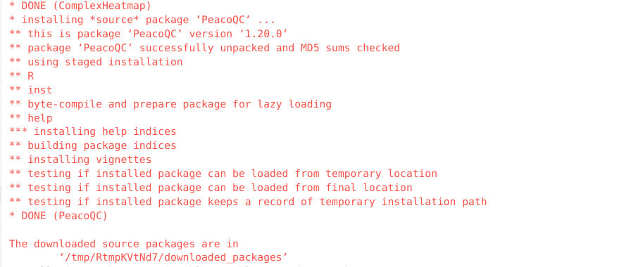
And finally, once all the dependencies are installed, PeacoQC starts to install.

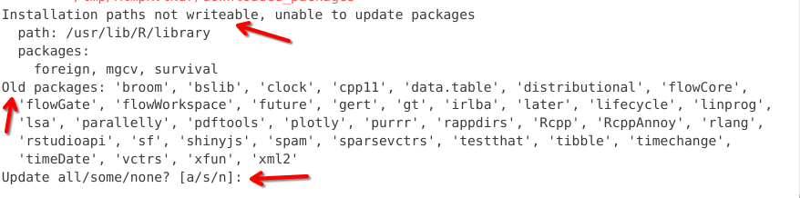
Occasionally, during installation, you will see a pop-up windown like this one in the console. This let’s you know that some of the package dependencies have newer updated versions that are available to download. We are prompted to select between updating all, some or none. You will need to specify via the console how you want to proceed, by typing and entering one of the suggested options [a/s/n].

Alternatively you may encounter a pop-up that resembles this one. Unlike the a/s/n output, we would need to provide a number for our intended choice. In this case, I went ahead and skipped all updates by typing 3 into the console, then hitting enter.

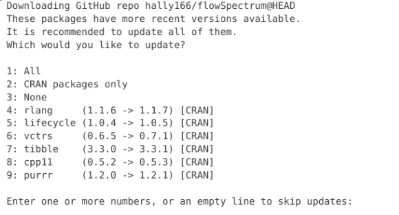
Generally, it’s okay to update if you have the time. Updates generally consist of minor improvements or bug fixes, that shouldn’t cause major issues. If you are short on time, you can go ahead and select skip the update by entering the value (n) for the none option.

With PeacoQC has been installed, we can load it via the library() call

Tip

Remeber, library() doesn’t require ” ”

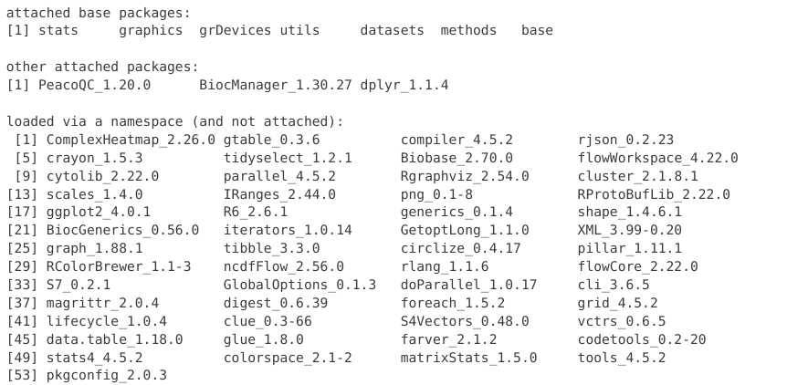
library(PeacoQC)

And we can check to see if it has been attached to the local environment

sessionInfo()

R version 4.5.2 (2025-10-31)
Platform: x86_64-pc-linux-gnu
Running under: Debian GNU/Linux 13 (trixie)

Matrix products: default
BLAS:   /usr/lib/x86_64-linux-gnu/blas/libblas.so.3.12.1 
LAPACK: /usr/lib/x86_64-linux-gnu/lapack/liblapack.so.3.12.1;  LAPACK version 3.12.0

locale:
 [1] LC_CTYPE=en_US.UTF-8       LC_NUMERIC=C              
 [3] LC_TIME=en_US.UTF-8        LC_COLLATE=en_US.UTF-8    
 [5] LC_MONETARY=en_US.UTF-8    LC_MESSAGES=en_US.UTF-8   
 [7] LC_PAPER=en_US.UTF-8       LC_NAME=C                 
 [9] LC_ADDRESS=C               LC_TELEPHONE=C            
[11] LC_MEASUREMENT=en_US.UTF-8 LC_IDENTIFICATION=C       

time zone: America/New_York
tzcode source: system (glibc)

attached base packages:
[1] stats     graphics  grDevices utils     datasets  methods   base     

other attached packages:
[1] PeacoQC_1.20.0      BiocManager_1.30.27 BiocStyle_2.38.0   

loaded via a namespace (and not attached):
 [1] generics_0.1.4        shape_1.4.6.1         digest_0.6.39        
 [4] magrittr_2.0.4        evaluate_1.0.5        grid_4.5.2           
 [7] RColorBrewer_1.1-3    iterators_1.0.14      circlize_0.4.17      
[10] fastmap_1.2.0         foreach_1.5.2         doParallel_1.0.17    
[13] jsonlite_2.0.0        graph_1.88.1          GlobalOptions_0.1.3  
[16] ComplexHeatmap_2.26.0 flowWorkspace_4.22.1  scales_1.4.0         
[19] XML_3.99-0.20         Rgraphviz_2.54.0      codetools_0.2-20     
[22] cli_3.6.5             RProtoBufLib_2.22.0   rlang_1.1.7          
[25] crayon_1.5.3          Biobase_2.70.0        yaml_2.3.12          
[28] otel_0.2.0            cytolib_2.22.0        ncdfFlow_2.56.0      
[31] tools_4.5.2           parallel_4.5.2        dplyr_1.1.4          
[34] colorspace_2.1-2      ggplot2_4.0.1         GetoptLong_1.1.0     
[37] BiocGenerics_0.56.0   vctrs_0.7.1           R6_2.6.1             
[40] png_0.1-8             matrixStats_1.5.0     stats4_4.5.2         
[43] lifecycle_1.0.5       flowCore_2.22.1       S4Vectors_0.48.0     
[46] htmlwidgets_1.6.4     IRanges_2.44.0        clue_0.3-66          
[49] cluster_2.1.8.1       pkgconfig_2.0.3       pillar_1.11.1        
[52] gtable_0.3.6          data.table_1.18.2.1   glue_1.8.0           
[55] xfun_0.56             tibble_3.3.1          tidyselect_1.2.1     
[58] knitr_1.51            farver_2.1.2          rjson_0.2.23         
[61] htmltools_0.5.9       rmarkdown_2.30        compiler_4.5.2       
[64] S7_0.2.1

As you may have noticed, the section of loaded via namespace (but not attached) packages has grown larger. These packages are dependencies for the attached packages (dplyr, BiocManager and PeacoQC). Since the functions within these dependencies are only used selectively by the attached packages, they do not need to be active within the local environment.

To see what packages are installed (but not yet loaded), we can use the installed.packages() function to return a list of R packages for your computer.

installed.packages()

Install from GitHub

In addition to the CRAN and Bioconductor repositories, individual R packages can also be found on GitHub hosted on their respective developers GitHub accounts. Newer packages that are still being worked on (often in the process of submission to CRAN or Bioconductor) can be found here, as well as those where the author decided not to bother with a review process, and just made the packages immediately available, warts and all.

While many gems of R packages can be found on GitHub, there are also a bunch of R packages that due to deprecation since when they were published and released have stopped working. This is often the case for R packages that are not maintained, which is why it’s useful to check the commits and issues pages to see when the last contribution occurred. We will take a closer look at how to do so later on.

To install packages from GitHub, you will need the remotes package, which can be found on CRAN.

Spot Check #1

To install a package from CRAN, what function would you use? Click on the code-fold arrow below to reveal the answer.

Code

install.packages("remotes")

With the remotes package now installed, we can attach it to our local environment.

Spot Check #2

What function would be used to do so?

Code

library(remotes)

And finally, we can use the install_github() function to download R packages from the invidual developers GitHub account.

Spot Check #3

How would you look up the help documentation for this function?

Code

# Either by hovering over it within Positron or via

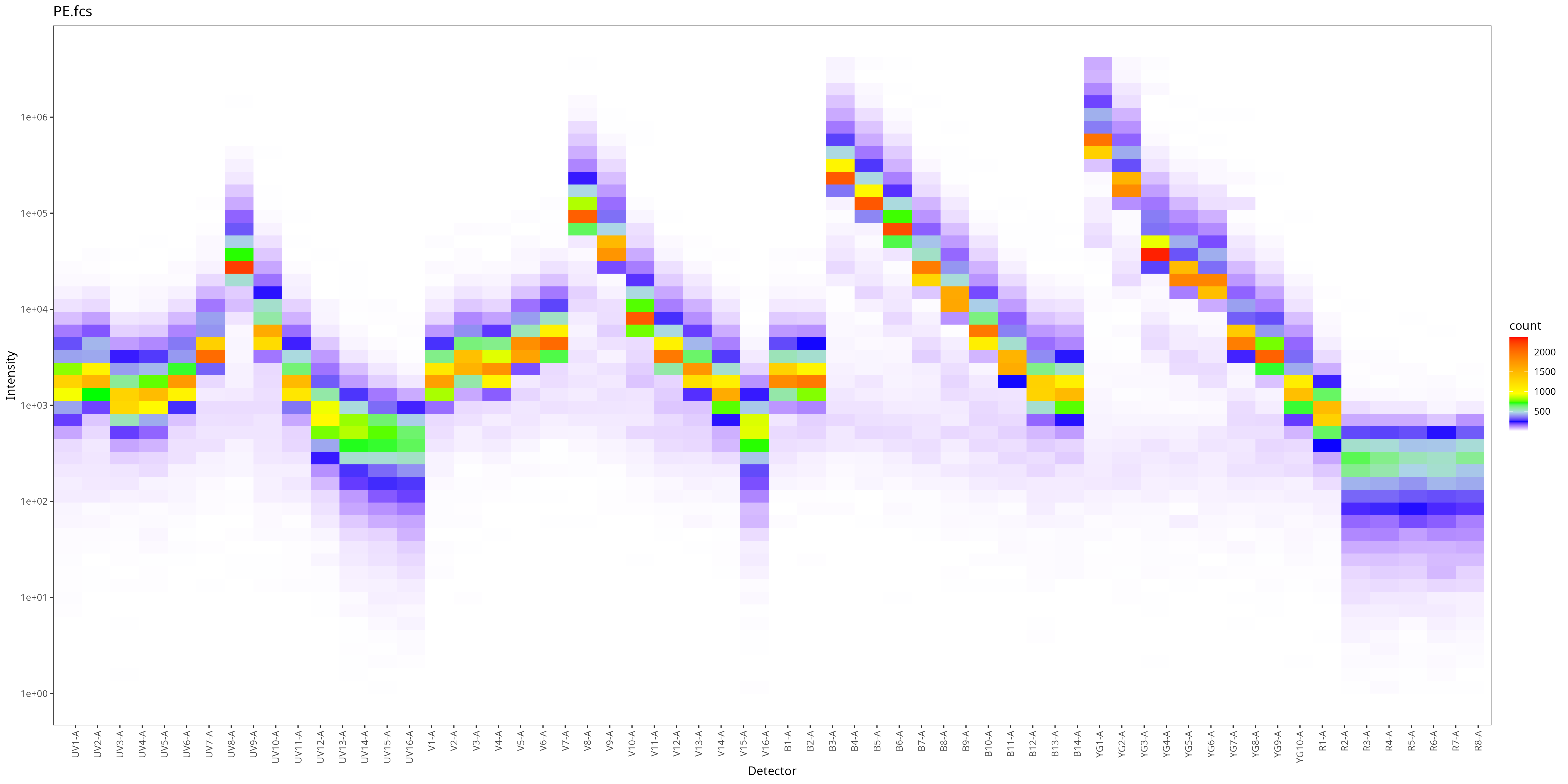
?install_github()

We will be installing a small R package flowSpectrum for this example. It’s one of the packages created by Christopher Hall, whose small series of Flow Cytometry Data Analysis in R tutorials were immensely useful when I was first getting started learning R. flowSpectrum can be used to generate spectrum-style plots for spectral flow cytometry data.

To install an R package from GitHub, we first need the GitHub username (so hally166 in this case), which is followed by a “/”, and then the name of the package repository (so flowSpectrum in this case). Our code should consequently be:

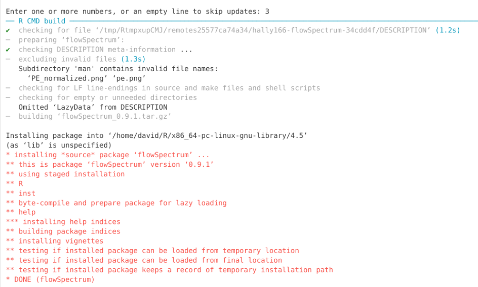
install_github("hally166/flowSpectrum")

When installing from GitHub, the opening installation scrawl will look different. Unlike R packages from CRAN or Bioconductor, which are usually shipped in an assembled binary format, R packages from GitHub start off as source code. So the first steps shown in the scrawl are the process of converting them to binary before proceeding.

This process of building R packages from source code is one of the reasons we needed to install Rtools (for Windows users) or Xcode Developer Tools (for MacOS) for this course. We will look at this topic in greater depth later in the course when we talk about creating R packages.

Troubleshooting Install Errors

We have now installed three R packages, dplyr, PeacoQC, and flowSpectrum. In my case, I did not encounter any errors during the installation. However, sometimes a package installation will fail due to an error encountered during the installation process. This can be due to a number of reasons, ranging from a missing dependency, or an update that caused a conflict. While these can occur for CRAN or Bioconductor packages, they are more frequently seen for GitHub packages where the Description/Namespace files may not have been fully updated yet to install all the required dependencies.

When encountering an error, start of by first reading through the message to see if you can parse any useful information about what package failed to install, and if it list the missing dependency packages name. The later was the case in the error message example shown below.

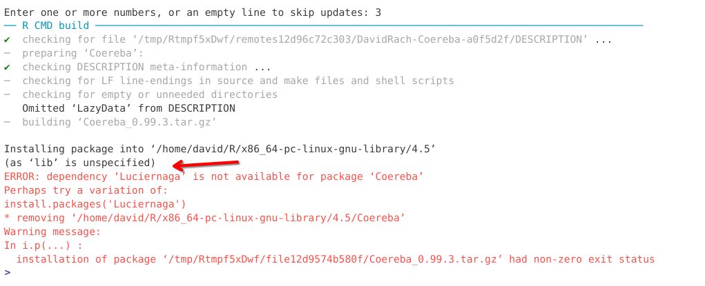
If you encounter an installation error this week, please take screenshots of the error message and post them to this Discussion. This will help us troubleshoot your installation, as well as provide additional examples of installation errors that will be used to update this section in the future.

Installing Specific-Package Versions

While we may be tempted to think of R packages as static, they change quite often, as their develipers add new features, fix bugs, etc. To help keep track of these changes (essential for reproducibility and replicability), R packages have version numbers.

When we run sessionInfo(), we can see an example of this, with the version number appearing after the package name.

sessionInfo()

R version 4.5.2 (2025-10-31)
Platform: x86_64-pc-linux-gnu
Running under: Debian GNU/Linux 13 (trixie)

Matrix products: default
BLAS:   /usr/lib/x86_64-linux-gnu/blas/libblas.so.3.12.1 
LAPACK: /usr/lib/x86_64-linux-gnu/lapack/liblapack.so.3.12.1;  LAPACK version 3.12.0

locale:
 [1] LC_CTYPE=en_US.UTF-8       LC_NUMERIC=C              
 [3] LC_TIME=en_US.UTF-8        LC_COLLATE=en_US.UTF-8    
 [5] LC_MONETARY=en_US.UTF-8    LC_MESSAGES=en_US.UTF-8   
 [7] LC_PAPER=en_US.UTF-8       LC_NAME=C                 
 [9] LC_ADDRESS=C               LC_TELEPHONE=C            
[11] LC_MEASUREMENT=en_US.UTF-8 LC_IDENTIFICATION=C       

time zone: America/New_York
tzcode source: system (glibc)

attached base packages:
[1] stats     graphics  grDevices utils     datasets  methods   base     

other attached packages:
[1] PeacoQC_1.20.0      BiocManager_1.30.27 BiocStyle_2.38.0   

loaded via a namespace (and not attached):
 [1] generics_0.1.4        shape_1.4.6.1         digest_0.6.39        
 [4] magrittr_2.0.4        evaluate_1.0.5        grid_4.5.2           
 [7] RColorBrewer_1.1-3    iterators_1.0.14      circlize_0.4.17      
[10] fastmap_1.2.0         foreach_1.5.2         doParallel_1.0.17    
[13] jsonlite_2.0.0        graph_1.88.1          GlobalOptions_0.1.3  
[16] ComplexHeatmap_2.26.0 flowWorkspace_4.22.1  scales_1.4.0         
[19] XML_3.99-0.20         Rgraphviz_2.54.0      codetools_0.2-20     
[22] cli_3.6.5             RProtoBufLib_2.22.0   rlang_1.1.7          
[25] crayon_1.5.3          Biobase_2.70.0        yaml_2.3.12          
[28] otel_0.2.0            cytolib_2.22.0        ncdfFlow_2.56.0      
[31] tools_4.5.2           parallel_4.5.2        dplyr_1.1.4          
[34] colorspace_2.1-2      ggplot2_4.0.1         GetoptLong_1.1.0     
[37] BiocGenerics_0.56.0   vctrs_0.7.1           R6_2.6.1             
[40] png_0.1-8             matrixStats_1.5.0     stats4_4.5.2         
[43] lifecycle_1.0.5       flowCore_2.22.1       S4Vectors_0.48.0     
[46] htmlwidgets_1.6.4     IRanges_2.44.0        clue_0.3-66          
[49] cluster_2.1.8.1       pkgconfig_2.0.3       pillar_1.11.1        
[52] gtable_0.3.6          data.table_1.18.2.1   glue_1.8.0           
[55] xfun_0.56             tibble_3.3.1          tidyselect_1.2.1     
[58] knitr_1.51            farver_2.1.2          rjson_0.2.23         
[61] htmltools_0.5.9       rmarkdown_2.30        compiler_4.5.2       
[64] S7_0.2.1

Alternatively, we can retrieve the same information for the individual packages via the packageVersion() function

packageVersion("PeacoQC")

[1] '1.20.0'

As well as from the citation() function.

citation("PeacoQC")

To cite package 'PeacoQC' in publications use:

  Emmaneel A (2025). _PeacoQC: Peak-based selection of high quality
  cytometry data_. doi:10.18129/B9.bioc.PeacoQC
  <https://doi.org/10.18129/B9.bioc.PeacoQC>, R package version 1.20.0,
  <https://bioconductor.org/packages/PeacoQC>.

A BibTeX entry for LaTeX users is

  @Manual{,
    title = {PeacoQC: Peak-based selection of high quality cytometry data},
    author = {Annelies Emmaneel},
    year = {2025},
    note = {R package version 1.20.0},
    url = {https://bioconductor.org/packages/PeacoQC},
    doi = {10.18129/B9.bioc.PeacoQC},
  }

How does a version number work? Lets say we have the following version number: 1.20.0

The first number of the version (1. in this case) denotes major changes, primarily those where after the version change the package may not be compatible with the code used in the prior version. As a consequence, this number changes rarely.

The second number (.20. in this case) is the minor version. Minor changes typically consist of new features that are added, that don’t affect the overall package function. These will change more frequently, especially for Bioconductor packages with fixed release cycles.

The final number (.0 in this case) is often used to denote small changes occuring within a minor release period, often bug-fixes or fixing typos within the documentation.

We may in the future need to install specific package versions (but wont be doing so today). As expected, which repository contains the R package influences how we would go about doing this.

For CRAN packages, we can use the remotes packages install_version() function. This allows us to provide the version number, and designate the repository location (the CRAN url in this case).

remotes::install_version("ggplot2", version = "3.5.2", repos = "https://cloud.r-project.org")

For GitHub-based R packages, the package versioning schema is not as strict as that of CRAN or Bioconductor. Typically, changes in R packagaes are put out by their developers as releases. When trying to install a particular release, we can add an additional argument to the install_github() function, specifying the release version’s tag number. For example:

remotes::install_github("DavidRach/Luciernaga", ref = "v0.99.7")

Alternatively, if the developer doesn’t implement releases, you can provide the hash number of a particular commit.

remotes::install_github("DavidRach/Luciernaga", ref = "8d1d694")

Documentation and Websites

We have already seen a couple ways to access the help documentation contained within an R package via Positron. Beyond internal documentation, R packages often have external websites that contain additional walk-through articles (ie. vignettes) to better document how to use the package.

For CRAN-based packages, we can start off by searching for the package name. So, in the case of dplyr:

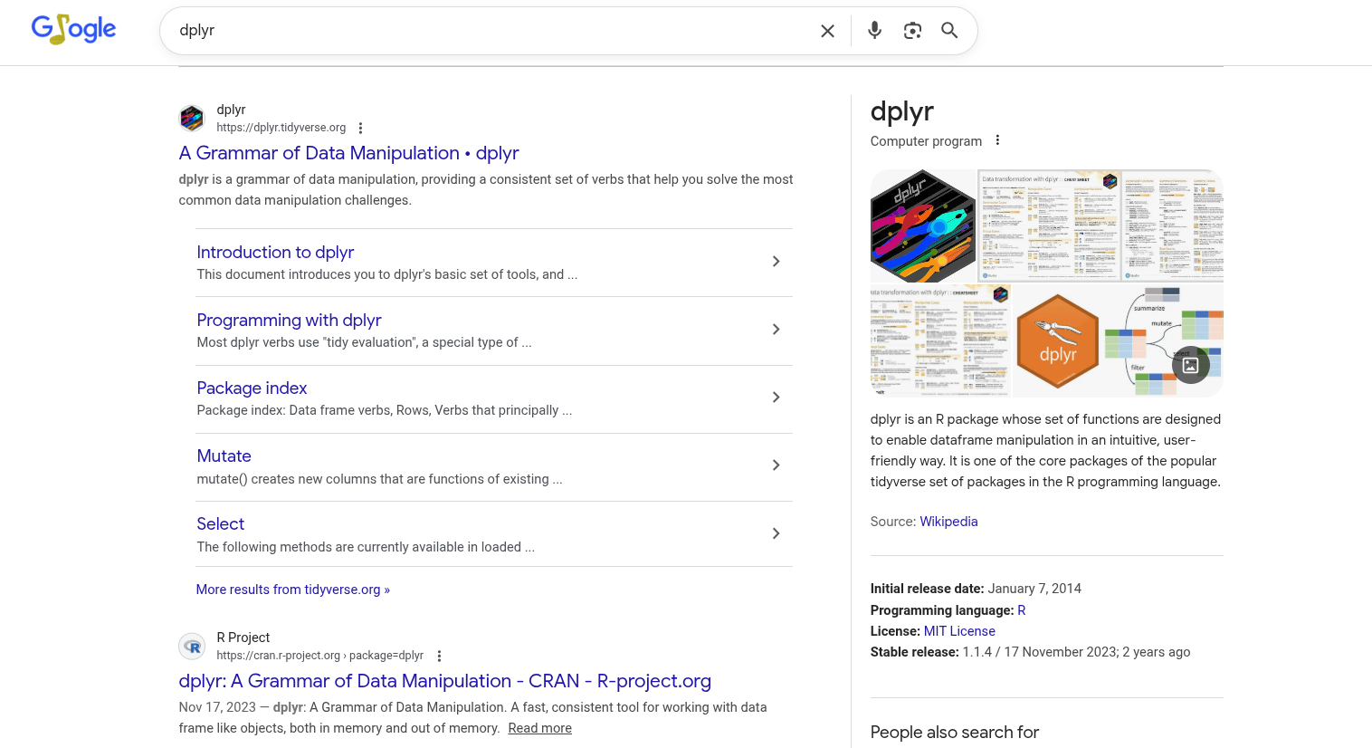
Two main suggestions pop up. One is the package’s CRAN page. Unfortunately, this one is not particularly user-friendly, although some text-based vignettes are accessible.

Because of this, many CRAN-based R packages (especially those part of the tidyverse) use pkgdown-generated websites hosted via a GitHub page (similar to the one used by this course. The second option on the search is dplyr’s pkgdown-style website

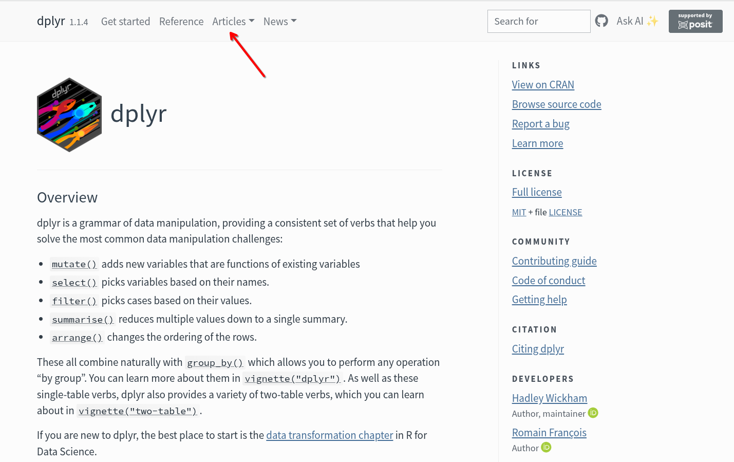
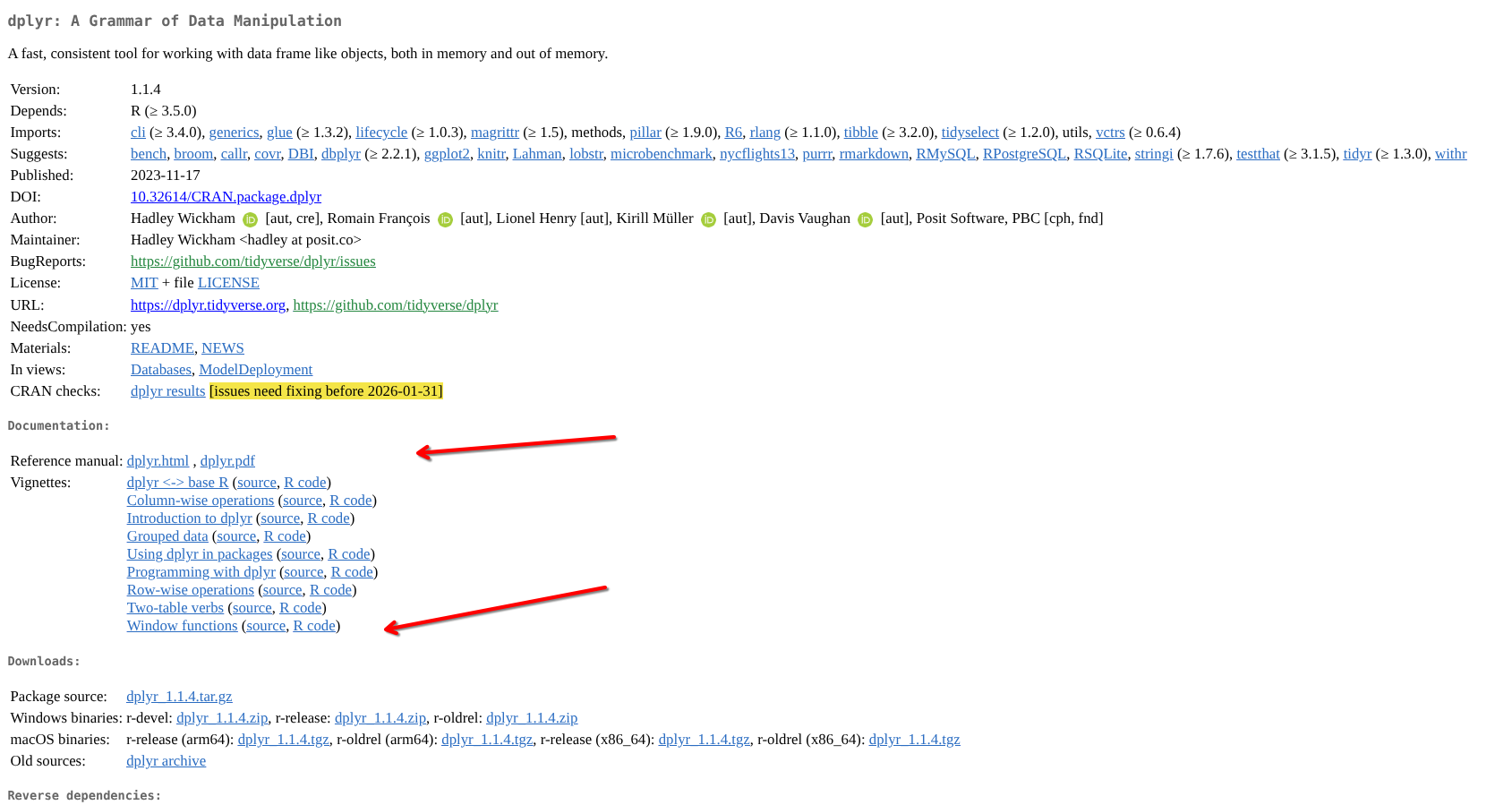
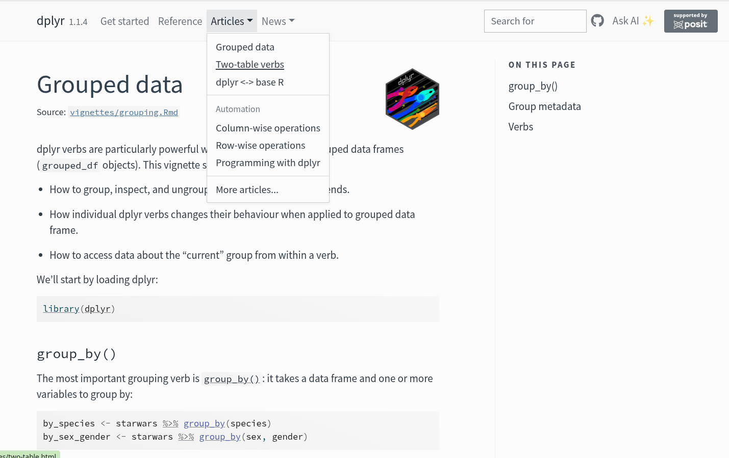
We can usually find the list of functions under the Reference tab, with the more extensive documentation vignettes being found under the Articles tab.

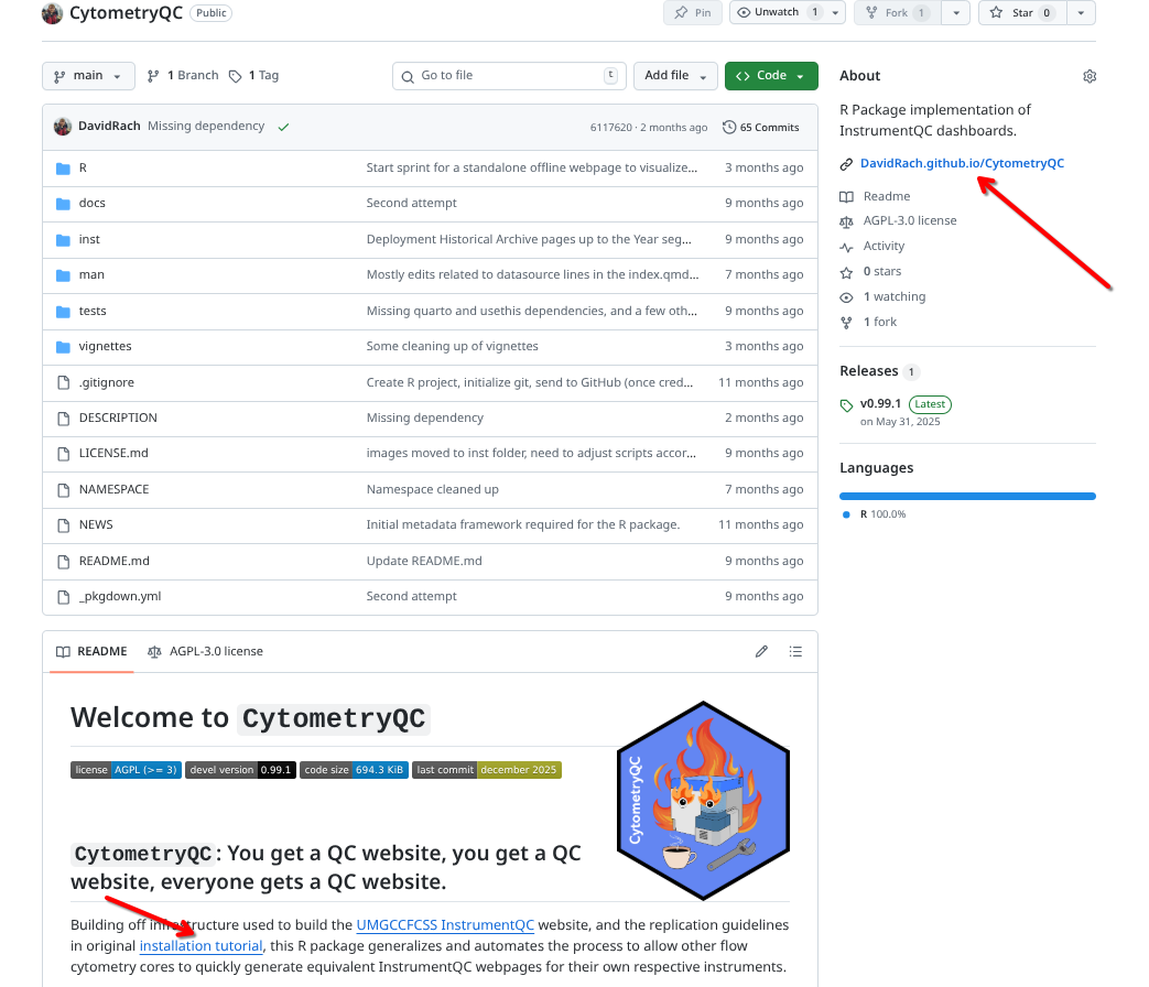
GitHub-based packages will vary depending on their individual developers, but often will also use pkgdown-style websites. These often appear as links on the right-hand side, or within the repository’s ReadMe.

For Bioconductor-based packages, on the package’s page we can typically find the already rendered vignette articles, usually as either html or pdf files. For example, with PeacoQC:

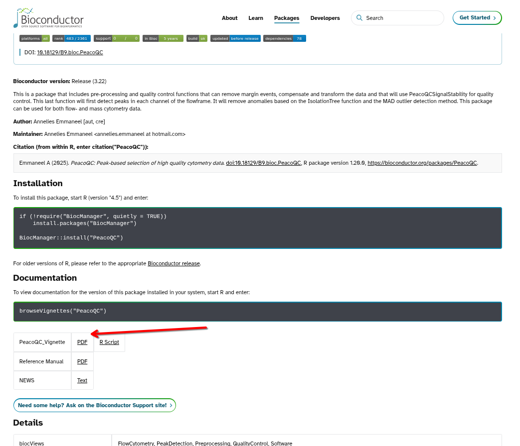
Additionally, package vignettes can also be reached via the packages help index page. These will usually appear under User guides, package vignettes, and other documentation.

Your Turn

Alright, we have now gone through the process of installing an R package from CRAN, Bioconductor, and GitHub. We will now install 20 other R packages we will need throughout the rest of the course.

Note

To make this interactive, I will task you to apply the previous concepts to figure out whether the packages need to be installed via CRAN, Bioconductor or GitHub.

Important

Feel free to view the website version to avoid accidental spoilers from the copied over index.qmd file. Alternatively, you can attempt to switch from the Source view to Visual Mode by right clicking with your mouse and selecting that option.

Tip

Start by searching each packages name. See if you can spot first either a CRAN or a Bioconductor website. Then enter the respective installation command (install.packages(), install(), install_github()) for the appropiate repository, add the package name, and run the code to see if the installation proceeds.

For cases where you are truly stuck, expand the code-fold below each package name to see the answer.

Note

Some of these packages may be dependencies of each other and may wind up installed before you get to them. If that is the case, no need to reinstall, count it as a win, and proceed to the next R package.

Remember,if you encountered any installation errors in the process, please take screenshots and post them on the the Discussion page to help with improved documentation.

1/20

R package: purrr

Code

# Location: CRAN
# Website: https://purrr.tidyverse.org/

install.packages("purrr")

2/20

R package: flowCore

Code

# Location: Bioconductor
# Website: https://www.bioconductor.org/packages/release/bioc/html/flowCore.html

install("flowCore")

3/20

R package: flowWorkspace

Code

# Location: Bioconductor
# Website: https://www.bioconductor.org/packages/release/bioc/html/flowWorkspace.html

install("flowWorkspace")

4/20

R package: stringr

Code

# Location: CRAN
# Website: https://stringr.tidyverse.org/

install.packages("stringr")

5/20

R package: ggplot2

Code

# Location: CRAN
# Website: https://ggplot2.tidyverse.org/

install.packages("ggplot2")

6/20

R package: ggcyto

Code

# Location: Bioconductor
# Website: https://www.bioconductor.org/packages/release/bioc/html/ggcyto.html

install.packages("ggcyto")

7/20

R package: tidyr

Code

# Location: CRAN
# Website: https://tidyr.tidyverse.org/

install.packages("tidyr")

8/20

R package: openCyto

Code

# Location: Bioconductor
# Website: https://www.bioconductor.org/packages/release/bioc/html/openCyto.html

install.packages("openCyto")

9/20

R package: FlowSOM

Code

# Location: Bioconductor
# Website: https://www.bioconductor.org/packages/release/bioc/html/FlowSOM.html

install.packages("FlowSOM")

10/20

R package: xml2

Code

# Location: CRAN
# Website: https://xml2.r-lib.org/

install.packages("xml2")

11/20

R package: saeyslab/CytoNorm

Code

# Location: GitHub
# Website: https://github.com/saeyslab/CytoNorm

install_github("saeyslab/CytoNorm")

12/20

R package: lubridate

Code

# Location: CRAN
# Website: https://lubridate.tidyverse.org/

install.packages("lubridate")

13/20

R package: httr2

Code

# Location: CRAN
# Website: https://httr2.r-lib.org/

install.packages("httr2")

14/20

R package: flowGate

Code

# Location: Bioconductor
# Website: https://www.bioconductor.org/packages/release/bioc/html/flowGate.html

install("flowGate")

15/20

R package: devtools

Code

# Location: CRAN
# Website: https://devtools.r-lib.org/

install.packages("devtools")

16/20

R package: plotly

Code

# Location: CRAN
# Website: https://plotly.com/r/getting-started/

install.packages("plotly")

17/20

R package: biosurf/cyCombine

Code

# Location: GitHub
# Website: https://github.com/biosurf/cyCombine

install_github("biosurf/cyCombine")

18/20

R package: CytoML

Code

# Location: Bioconductor
# Website: https://www.bioconductor.org/packages/release/bioc/html/CytoML.html

install("CytoML")

19/20

R package: Rtsne

Code

# Location: CRAN
# Website: https://github.com/jkrijthe/Rtsne

install.packages("Rtsne")

20/20

R package: uwot

Code

# Location: CRAN
# Website:https://jlmelville.github.io/uwot/

install.packages("uwot")

Congratulations! You have (hopefully) survived the package installation onslaught that is Week #1 of the course.

Remember to submit any encountered installation error screenshots to the Discussion page.

Wrap-Up

In this session, we walked through what are R packages, where to find them, how to install them, and a bit about troubleshooting any installation errors you may encounter during the process.

You then proceeded to install most of the R packages that you would need throughout the Cytometry in R course. These included tidyverse packages from the CRAN repository used for working with data structures and plots, as well as more cytometry focused R packages from Bioconductor repository.

If you have any questions, or want to discuss this week’s topics in more depth with the other course participants, please head over to the Discussion page and open a new topic.

Next week, we will start learning about file paths, by which we will be able to tell our computer where to find your fcs files, how to retrieve the file names, subset those that may be of particular interest, and copy them over to a new folder. In the processs, we will learn a little more about how variables, objects, and list work within R.

Until then, Best Wishes!

David

Additional Resources

Tidy Tales An useful beginner-friendly blogpost covering additional aspects from a different perspective.

Introduction to Bioconductor A talk by Martin Morgan with more information about the Bioconductor project.

R Packages A book by Hadley Wickham and Jennifer Bryan, covering all the different internals of R packages.

Take-home Problems

Below you will find the optional take-home problems for Week #1. Learning how to code well requires continous practice, and that involves cycles of trying something, failing, and troubleshooting to get it working. The goal of these problems is to help you explore the topic in greater depth than the currated boundaries of this one lecture.

You are more than welcome to open a Discussion to engage with others in the course to discuss these questions. Once you are done tinkering, and want to get final instructor feedback on your work, place your files within a folder, and follow the instructions to submit it as a Pull Request to the Cytometry In R repositories homework branch.

Problem 1

We installed PeacoQC during this session, but we didn’t have time to explore what functions are present within the package. Using what you have learned about accessing documentation, figure out and list what functions it contains

Problem 2

Take a closer look at the list of Bioconductor cytometry packages. Report back on how many there are currently in Bioconductor, the author/maintainer with the most contributed cytometry R packages, and a couple packages that you would be interested in exploring more in-depth later in the course.

Problem 3

There is another way to install R packages, using the newer pak package. Positron uses this when installing suggested dependencies.

After learning more about it via the documentation and it’s pkgdown website, I would like you to attempt to install the following three R packages using this newer method: “broom”, “cytoMEM”, “DillonHammill/CytoExploreR”.

Take screenshots, and in a new quarto markdown document, describe how the installation process differed from what you saw for install.packages(), install() and install_github().