03 - Inside an FCS File
2026-02-16

![]()
![]()
Background
.
Welcome to the Week #3! Having subjected everyone to two R-focused weeks, this week will have more of a cytometry-focus as we slice into an .fcs file.
We will hopefully gather greater understanding of how an .fcs file is structured and what additional kinds of information we can retrieve (while becoming increasingly puzzled why different manufacturers insist on using different keyword names for the exact same things).
.
We will also gain additional exposure to more object types in R (vectors, list, matrices and data.frames).
Continuing the analogy from last week, if every function is the equivalent of a tool in a toolbox, each tool requires certain types of things to do its job properly (hammer ~ nail, screwdriver ~ screws, paintbrush ~ paint, etc.).
Being able to identify what type/kind of object a particular variable we have created in R is will allow us to pass it to the correct function that will allow us to work with that object type.
Housekeeping
We are building off concepts that were covered in Week #1 (Installing R packages) and especially Week #2 (File Paths). For those who are flow cytometry beginners, please see UChicago Flow Flow Basics Series for additional context.
Today’s Goal
If you find yourself at some point going “I have no idea what is going on”, please pause, take a break, and circle back later in the day. Our goal is not to have you memorize how to quickly access 100 archaic keywords, but rather showcase a typical object exploration workflow.
So don’t power through, but rather circle back when you are in an exploring mindset. Consider what kind of information from within an .fcs file you’d like to retrieve, and then explore/navigate your way through the various paths until you find the information that you were looking for.
Housekeeping
As we do every week, on GitHub, sync your forked-version of the CytometryInR course to bring in the most recent updates. Then within Positron, pull in those changes to your local computer. From there, copy the data folder to a separate project folder you have created. This will prevent any merge issues bringing in new data next week.
For YouTube walkthrough of this process, click here
Walk Through
Getting Set Up
Set up File Paths
.
Having copied over the new data to your working project folder (Week 3 or whatever your chosen name), let’s identify the file paths between our working directory and the fcs files. If you retained the same project organization structure we had during Week #2, it may look similar to the following:
Locate .fcs files
.
We will now locate our .fcs files. As we saw last week, our computer will need the full file.paths to these individual files, so we will set the list.files() “full.names” argument to TRUE.
.
By contrast, if the “full.names” argument was set to FALSE, we would have retrieved just the file names
.
This would have been the equivalent of running the basename function on the “full.names=TRUE” output.
flowCore
.
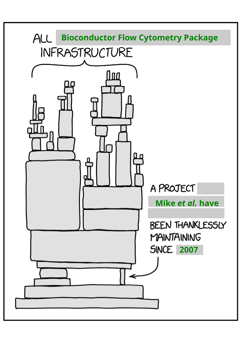
We will be using the flowCore package, which is the oldest and most-frequently downloaded flow cytometry package on Bioconductor.
.
flowCore is also one of the many Bioconductor packages maintained by Mike Jiang. In many ways (as those who completed the optional take-home problems for Week #1 know) reminiscent of this xkcd comic:
.
As with all our R packages, we first need to make sure flowCore is attached to our local environment via the library call.
.
The function we will be using today is the read.FCS() function. Do you remember how to access the help documentation?
.
To start, lets select just the first .fcs file. We will do this by indexing the first item within fcs_files via the square brackets [].
flowFrame
.
For read.FCS(), it accepts several arguments. The argument “filename” is where we provide our file.path to .fcs file that we wish to load into R. Let’s go ahead and do so
.
Please note, if you are doing this with your own .fcs files, you will need to provide two additional arguments, “transformation” = FALSE, and “truncate_max_range” = FALSE for the files to be read in correctly. We will revisit the reasons why in Week #5.
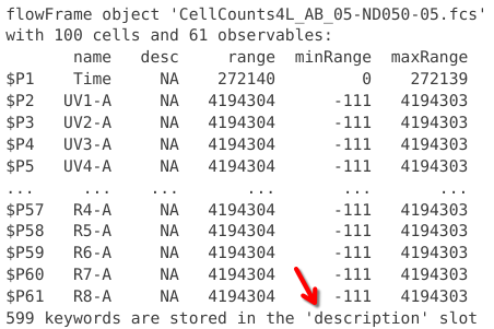
flowFrame object 'CellCounts4L_AB_05-ND050-05.fcs'
with 100 cells and 61 observables:
       name   desc     range  minRange  maxRange
$P1    Time     NA    272140         0    272139
$P2   UV1-A     NA   4194304      -111   4194303
$P3   UV2-A     NA   4194304      -111   4194303
$P4   UV3-A     NA   4194304      -111   4194303
$P5   UV4-A     NA   4194304      -111   4194303
...     ...    ...       ...       ...       ...
$P57   R4-A     NA   4194304      -111   4194303
$P58   R5-A     NA   4194304      -111   4194303
$P59   R6-A     NA   4194304      -111   4194303
$P60   R7-A     NA   4194304      -111   4194303
$P61   R8-A     NA   4194304      -111   4194303
476 keywords are stored in the 'description' slot
.
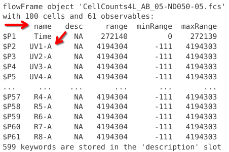
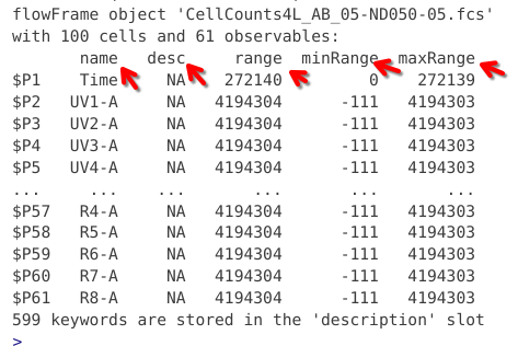
In this case, we can see the .fcs file has been read into R as a “flowFrame” object. We can also see the file name, as well as details about the number of cells, and number of columns (whether detectors (for raw spectral flow data) or fluorophores (for unmixed spectral flow data)).
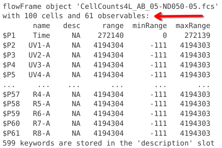
.
Directly below we see what resembles a table. At first glance, the only column with an immediately discernable purpose is the one with the name column, which is listing the detectors present on a Cytek Aurora.
.
And finally, at the bottom we reach a line that tells us that for this .fcs files, 599 keyword can be found in a description slot.
.
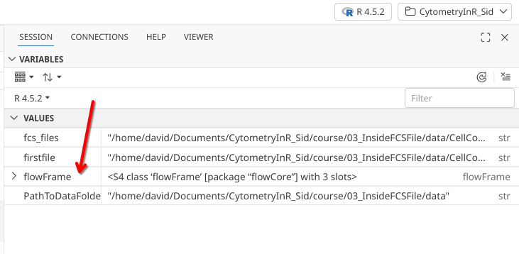
So let’s get our bearings, we have loaded in an .fcs file to R, but let’s use some of the concepts we covered last week to try to understand a bit about what type or class of object we are working with. From the output, we saw the words flowFrame object, so let’s read it back in again, but assign it to an variable/object called flowFrame so that we can use the type-discerning functions we worked with last week on.
.
As we create this variable, if we have the session tab selected on our right secondary side bar, we see it appear:
.
If we were to use the type-determining functions we learned last week
.
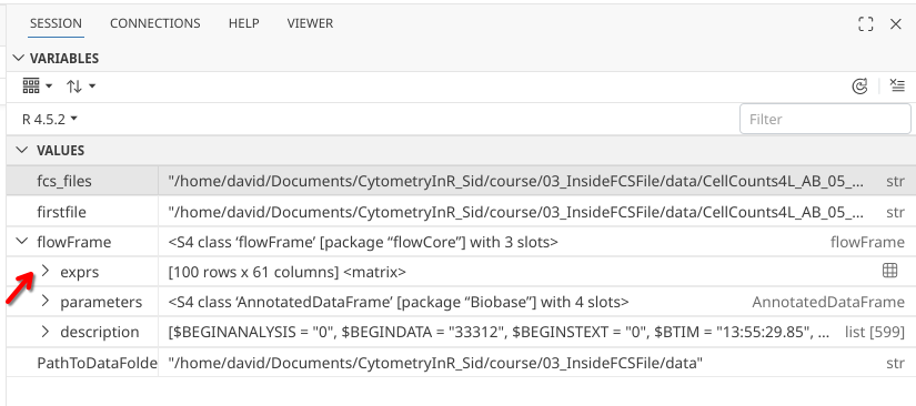
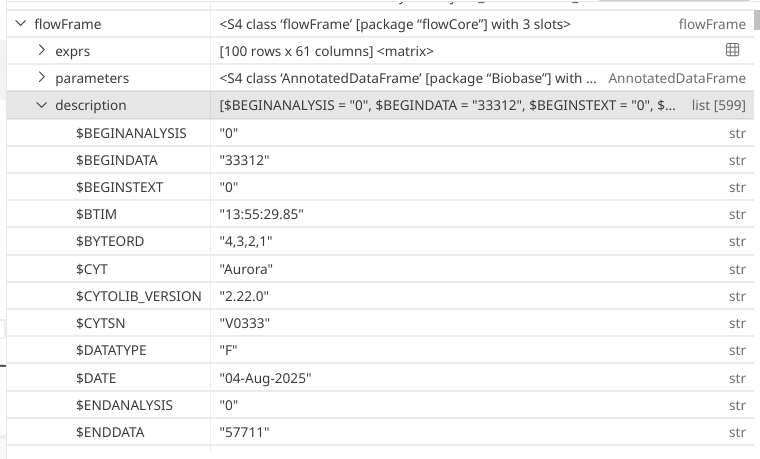
flowFrames are a class of object with a structure defined within the flowCore package. They are used to work with the data contained within individual .fcs files. Looking again at the right secondary side bar, we can see that it shows up as a ““S4 class flowFrame package flowCore”“” with 3 slots, with the words flowFrame adjacent to it.
.
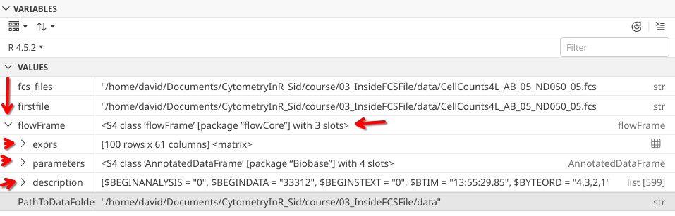
A perfectly valid first reaction to first reading this is “well how should I know what any of this means?”. Powering through this initial discomfort, let’s go ahead and click on the dropdown arrow next to the variables name and see if we get any additional clarity on the issue.
.
When we do so, three additional drop-downs appear. Based on the previous line that mentioned 3 slots, we could infer that each line corresponds to one of those slots.
.
What we are encountering with flowFrame is our first example of an S4 object type. These more-complicated object types are quite common for the various Bioconductor affilitated R packages.
.
These objects will usually appear with either S4 or S3 in their metadata, and are made up of various simpler object types that are cobbled together within the larger object, usually occupying individual slots.
.
What advantage this bundling provides will be something we revisit throughout the course as you encounter more of these S4/S3 objects.
exprs
.
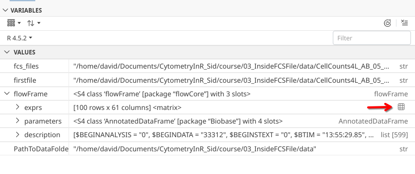
The first slot within the flowFrame object shows up with the name “exprs”. For the exprs object, glancing at it’s middle column, we can based on the 100 rows and 61 columns, that it is likely a matrix-style object. We might also recall we saw similar numbers in the printed output when we ran read.FCS()earlier.
.
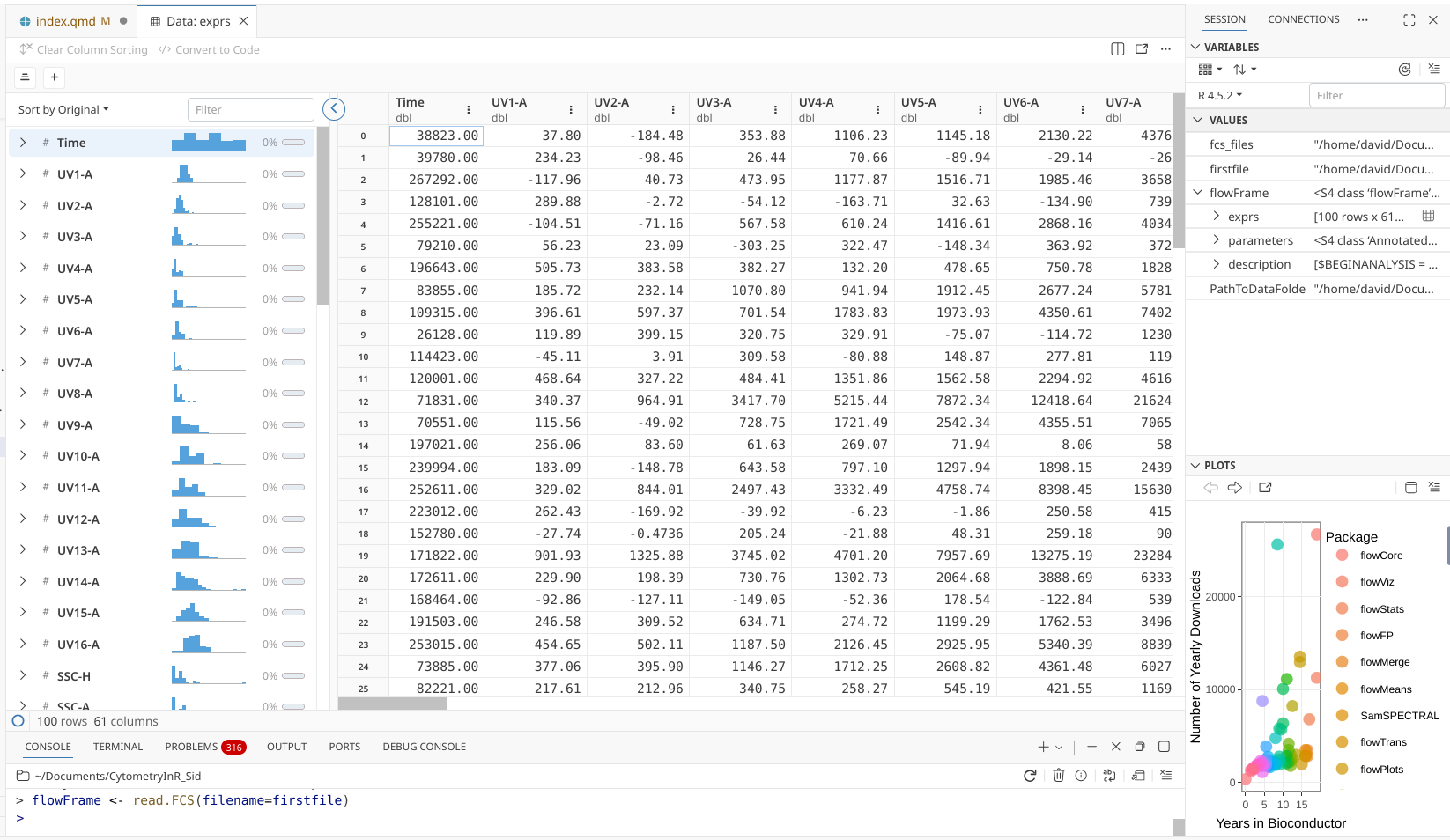
Which likely means that “exprs” slot is where the MFI data for the individual acquired cells within our .fcs file is being stored. Within Positron, for a matrix object, we can click on the little grid symbol on the far right to open up the table within editor.
.
If we utilize the scroll bars, we can see that the individual detectors (in the case of uploading a raw spectral fcs file, they would appear as fluorophores for unmixed spectral or conventional fcs files) occupy the individual columns, which are named. The rows are not named, but number 100, matching the number of cells present in the .fcs file. Additionally, on the far left there is a little summary table about the overall data.
.
Let’s go ahead and assign this matrix to a new variable/object so that we can explore it later. Since flowFrame is an S4 object, it’s slots can be individually accessed by adding the @ symbol and the respective slot name.
.
Alternatively, we can use the Bioconductor helper function exprs() to get data held in that slot
.
In the case of the above, this displayed text output to the console would be unwiedly to display all at once. If we wanted to only see the first five rows, we could use the head() function, and provide a value of 5.
       Time      UV1-A       UV2-A     UV3-A      UV4-A      UV5-A      UV6-A
[1,]  38823   37.79983 -184.479996 353.87714 1106.22998 1145.18140 2130.21899
[2,]  39780  234.23021  -98.456429  26.43876   70.65833  -89.93541  -29.14263
[3,] 267292 -117.96355   40.732426 473.94574 1177.86975 1516.70935 1985.46130
[4,] 128101  289.87671   -2.723389 -54.11960 -163.71489   32.62989 -134.90411
[5,] 255221 -104.50541  -71.163338 567.57562  610.23627 1416.61328 2868.16040
          UV7-A     UV8-A       UV9-A     UV10-A    UV11-A    UV12-A     UV13-A
[1,] 4376.34277 3246.7952 32050.65039  8123.2637 1992.5785 1070.3323  956.43573
[2,]  -26.34649 -162.6675    17.98848   271.9152  154.8575  163.5411  -32.81524
[3,] 3658.87671 4140.1724 59792.16406 14013.7969 3427.4324 1668.7588 1071.14636
[4,]  739.71960  402.9025   427.37534   315.6364 -223.0423  145.7121  127.03777
[5,] 4034.58789 3234.6626 40126.46484 10325.0371 1974.0907 1033.8450  -21.57245
        UV14-A    UV15-A    UV16-A  SSC-H      SSC-A      V1-A      V2-A
[1,]  290.8685 385.49921 670.97687 657613  750760.12 1171.1390  154.5628
[2,] -104.9198 103.41382  71.41528  83481   81552.85  266.2424  705.2527
[3,]  730.1430 214.93053 252.75406 890845 1183519.00 1196.0931 1183.1105
[4,] -207.8978 -55.37944 -45.10131  75103   72457.33  227.9926  556.9189
[5,]  273.6271 960.16290 341.20633 415791  501690.97  717.2498  929.9780
             V3-A      V4-A       V5-A      V6-A       V7-A        V8-A
[1,] 1346.4488525 1706.9260 1923.50940  898.2527 3162.55371  83596.5078
[2,]  244.3218689  341.0508  381.15939   87.1600  151.68785    119.5544
[3,] 2087.0092773  824.6352 1635.27258 1613.9069 4653.16260 176981.6094
[4,]   -0.8137281  205.4732   18.12125  179.6371  -69.50061   -132.4348
[5,] 1358.4512939  788.6506 1208.81006 1156.7040 3118.42627 104951.2578
           V9-A      V10-A        V11-A       V12-A      V13-A       V14-A
[1,] 32506.7617 27161.5137  6236.072754 2220.303223 2023.39966  753.589355
[2,]   -79.7691  -109.1783   -73.991196  114.375542  -11.53453  124.986206
[3,] 69236.4297 57626.8984 13175.838867 4534.874023 3434.38989 1995.172363
[4,]   129.2739   231.8918    -5.473321    8.792875  -24.62049   -8.212234
[5,] 42090.0781 34104.3164  7620.552734 3103.544189 2426.43359  650.836304
         V15-A     V16-A   FSC-H      FSC-A SSC-B-H   SSC-B-A      B1-A
[1,]  510.9540 228.34962 1055905 1217097.50  716733 815959.06  606.6683
[2,] -207.3494 -28.96272   79696   83439.11  104575 103132.83  195.2795
[3,] 1321.8030 615.05560 1092481 1453969.38  757351 982038.31 2010.5110
[4,] -133.7503 -34.32619   64760   60415.23   67955  66806.13 -146.8936
[5,]  290.2892 473.32599 1038362 1184479.00  425296 522873.12 1015.5981
           B2-A       B3-A        B4-A        B5-A        B6-A       B7-A
[1,]  416.98294  4172.4712 192400.0938  93929.9375  54236.3320 19342.6445
[2,]  333.25662   332.1675   -230.9639    196.7810    292.8945  -187.2845
[3,] 2150.21826 10106.9551 437801.5625 212176.1562 124294.3594 45068.3008
[4,]  -34.90987   165.7988    675.0156    136.3076    482.8665   133.0948
[5,]  639.77527  6034.0200 244022.6094 118871.4609  68616.9688 24067.7949
            B8-A       B9-A       B10-A       B11-A     B12-A     B13-A
[1,] 10507.24219  9498.1270  4465.50928 1668.048096 2199.9475 1581.7345
[2,]    70.90886  -334.3563   188.05545 -663.359619 -163.2331   27.9856
[3,] 24289.59180 22500.1914 10624.99219 4684.497559 3471.7749 2727.3904
[4,]   432.28091   246.8794   -94.44906    2.905877  106.8489  283.3633
[5,] 14182.12793 13019.7100  5577.33984 2753.355957 1279.3009 1423.0276
          B14-A      R1-A        R2-A       R3-A       R4-A       R5-A
[1,] 1487.56860  147.1335  129.867630   35.90353  267.23999   49.79849
[2,]  205.82298 -142.9224   66.516052  113.63218  -94.41375   98.13978
[3,] 2371.95850 -128.3749 -105.482544  726.48547   18.87000   95.47879
[4,]   33.24665  127.5455  122.607941   37.83584  -82.87500 -343.83768
[5,] 1565.72742 -266.4482   -3.350622 -178.39566 -117.10875 -100.10384
          R6-A       R7-A       R8-A
[1,] -732.7097   42.83144  248.56728
[2,]  143.4497 -263.28741  -85.83299
[3,] -194.4526  -84.08820 -301.46066
[4,]   82.3745   60.27896  -94.38461
[5,] -182.0066  184.36417  186.17207
.
This is much more workable, especially on a small laptop screen. We can see that there are names for each column corresponding to detector/fluorophore/metal depending on the .fcs file we are accessing. Lets retrieve these column names using the colnames() function.
     $P1N      $P2N      $P3N      $P4N      $P5N      $P6N      $P7N      $P8N
   "Time"   "UV1-A"   "UV2-A"   "UV3-A"   "UV4-A"   "UV5-A"   "UV6-A"   "UV7-A"
     $P9N     $P10N     $P11N     $P12N     $P13N     $P14N     $P15N     $P16N
  "UV8-A"   "UV9-A"  "UV10-A"  "UV11-A"  "UV12-A"  "UV13-A"  "UV14-A"  "UV15-A"
    $P17N     $P18N     $P19N     $P20N     $P21N     $P22N     $P23N     $P24N
 "UV16-A"   "SSC-H"   "SSC-A"    "V1-A"    "V2-A"    "V3-A"    "V4-A"    "V5-A"
    $P25N     $P26N     $P27N     $P28N     $P29N     $P30N     $P31N     $P32N
   "V6-A"    "V7-A"    "V8-A"    "V9-A"   "V10-A"   "V11-A"   "V12-A"   "V13-A"
    $P33N     $P34N     $P35N     $P36N     $P37N     $P38N     $P39N     $P40N
  "V14-A"   "V15-A"   "V16-A"   "FSC-H"   "FSC-A" "SSC-B-H" "SSC-B-A"    "B1-A"
    $P41N     $P42N     $P43N     $P44N     $P45N     $P46N     $P47N     $P48N
   "B2-A"    "B3-A"    "B4-A"    "B5-A"    "B6-A"    "B7-A"    "B8-A"    "B9-A"
    $P49N     $P50N     $P51N     $P52N     $P53N     $P54N     $P55N     $P56N
  "B10-A"   "B11-A"   "B12-A"   "B13-A"   "B14-A"    "R1-A"    "R2-A"    "R3-A"
    $P57N     $P58N     $P59N     $P60N     $P61N
   "R4-A"    "R5-A"    "R6-A"    "R7-A"    "R8-A"
.
Something interesting occurred when this occurred, we can see in addition to the detector names directly above each a “$P#N” pattern appear, with # standing for increasing numbers. If we recall, we saw something similar in the first output column when we first ran read.FCS().
.
Lets break out the str() and class() functions from last week and see what we can find out about why this is occuring.
.
In this case we can see that we don’t just have a vector (list) similar to what we saw with Fluorophores object last week, because instead of a chr [1:61] we get back a Named chr [1:61] designation. What we see is that in this case, each value has a corresponding index name as well. (ex. $P1N, $P2N, etc.) Let’s double check with class() function.
.
We can see that everything is character, but it doesn’t inform us that each index was named. This is one of the reasons it is best when trying to see what type of an object something is, to use multiple functions, to avoid missing some important details.
.
If we were trying to remove the names, being left with just the values (similar to what we saw with the vector-style list last week), we could use the unname() function:
 [1] "Time"    "UV1-A"   "UV2-A"   "UV3-A"   "UV4-A"   "UV5-A"   "UV6-A"
 [8] "UV7-A"   "UV8-A"   "UV9-A"   "UV10-A"  "UV11-A"  "UV12-A"  "UV13-A"
[15] "UV14-A"  "UV15-A"  "UV16-A"  "SSC-H"   "SSC-A"   "V1-A"    "V2-A"
[22] "V3-A"    "V4-A"    "V5-A"    "V6-A"    "V7-A"    "V8-A"    "V9-A"
[29] "V10-A"   "V11-A"   "V12-A"   "V13-A"   "V14-A"   "V15-A"   "V16-A"
[36] "FSC-H"   "FSC-A"   "SSC-B-H" "SSC-B-A" "B1-A"    "B2-A"    "B3-A"
[43] "B4-A"    "B5-A"    "B6-A"    "B7-A"    "B8-A"    "B9-A"    "B10-A"
[50] "B11-A"   "B12-A"   "B13-A"   "B14-A"   "R1-A"    "R2-A"    "R3-A"
[57] "R4-A"    "R5-A"    "R6-A"    "R7-A"    "R8-A"
.
Let’s return to the right sidebar to continue our exploration, by clicking on the dropdown arrow for exprs in the side-bar
.
The output is less user-friendly than what we saw when clicking on the little grid. If we scroll down far enough, we get down as far as [,61], which corresponds to the total number of columns.
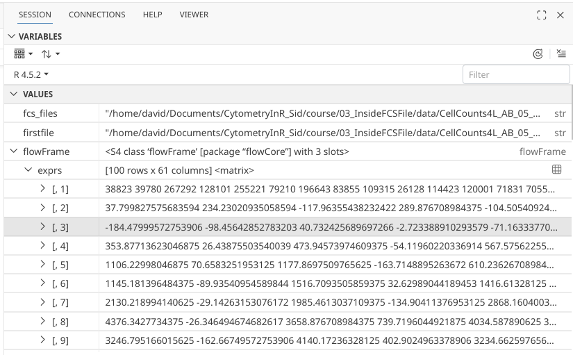
.
In base R, column order can be defined by placing the corresponding column index number after a comma “,”. So for this case, the first column would be designated would be [,1] while the last column would be designated [,61].
  [1]  38823  39780 267292 128101 255221  79210 196643  83855 109315  26128
 [11] 114423 120001  71831  70551 197021 239994 252611 223012 152780 171822
 [21] 172611 168464 191503 253015  73885  82221 176641 128533   4117 191632
 [31] 191229  58093 141776 265894  55593 227555 233212 248578  95165 171934
 [41]   1360 251847 195764 147503 118723   1060  90033 253553 268268  74610
 [51]  23531 150119 226391 201568 179264  79944 196686 252667 117309   3903
 [61]  77690 195142 229873 254472 179943 236618  68193  87154  28541  78622
 [71] 155664  50115  40866  70753 260118  12033  96149  20740  37461  73998
 [81] 231939 192329  88649 197664  86006 142486 159539 251298 104864 164090
[91] 102380 218968 145182 239323 261272 118979 17202 194277 229284 258723 [1] 248.567276 -85.832993 -301.460663 -94.384613 186.172073 -461.407745
[7] 843.507080 277.516113 -106.166855 281.633545 195.927261 818.865723
[13] 734.996460 209.356476 206.442596 279.859894 518.165222 56.947498
[19] 285.751007 857.126343 -94.384613 -213.030518 62.585236 138.409653
[25] 118.012444 328.255768 -61.635056 185.285233 464.384979 5.637739
[31] -66.385956 31.229273 1198.241211 185.475266 873.279419 457.607025
[37] -73.353951 37.880539 729.168640 221.772171 -169.512238 348.272888
[43] -338.391022 845.534119 -4.434176 620.024597 610.269409 -193.900208
[49] 230.830566 -23.754517 607.102112 14.949510 -34.333195 -169.132172
[55] -96.158287 220.631958 125.297165 -15.202891 -126.057304 193.393448
[61] 90.203819 -277.706146 590.505615 911.096619 -92.230873 347.259369
[67] 135.559113 369.430267 -62.015125 -180.597672 -146.517868 810.440796
[73] 134.038818 -165.268097 727.711731 -88.746880 62.901962 203.275330
[79] 436.196289 -242.676147 -40.857769 222.278946 -170.272385 525.513245
[85] -41.491222 176.670258 201.501648 175.530045 329.839386 474.140167
[91] -48.142490 -174.833252 46.052090 357.584656 -26.541714 191.493088
[97] 211.320190 124.790398 -113.324883 343.268616.
What would happen if used a column index number that didn’t exist? Let’s check.
.
We get back an error message telling us the subscript is out of bounds.
.
So if columns are specified by a number after the comma (ex. [,1]), how are rows specified? In R, rows would be specified by a number before the comma [1,]
         Time         UV1-A         UV2-A         UV3-A         UV4-A
  38823.00000      37.79983    -184.48000     353.87714    1106.22998
        UV5-A         UV6-A         UV7-A         UV8-A         UV9-A
   1145.18140    2130.21899    4376.34277    3246.79517   32050.65039
       UV10-A        UV11-A        UV12-A        UV13-A        UV14-A
   8123.26367    1992.57849    1070.33228     956.43573     290.86853
       UV15-A        UV16-A         SSC-H         SSC-A          V1-A
    385.49921     670.97687  657613.00000  750760.12500    1171.13904
         V2-A          V3-A          V4-A          V5-A          V6-A
    154.56281    1346.44885    1706.92603    1923.50940     898.25269
         V7-A          V8-A          V9-A         V10-A         V11-A
   3162.55371   83596.50781   32506.76172   27161.51367    6236.07275
        V12-A         V13-A         V14-A         V15-A         V16-A
   2220.30322    2023.39966     753.58936     510.95404     228.34962
        FSC-H         FSC-A       SSC-B-H       SSC-B-A          B1-A
1055905.00000 1217097.50000  716733.00000  815959.06250     606.66833
         B2-A          B3-A          B4-A          B5-A          B6-A
    416.98294    4172.47119  192400.09375   93929.93750   54236.33203
         B7-A          B8-A          B9-A         B10-A         B11-A
  19342.64453   10507.24219    9498.12695    4465.50928    1668.04810
        B12-A         B13-A         B14-A          R1-A          R2-A
   2199.94751    1581.73450    1487.56860     147.13348     129.86763
         R3-A          R4-A          R5-A          R6-A          R7-A
     35.90353     267.23999      49.79849    -732.70966      42.83144
         R8-A
    248.56728
.
And while not the focus of today, we could retrieve individual values from a matrix by specifying both a row and a column index number. So for example, if we wanted the MFI value for the UV1-A detector for the first acquired cell (knowing that UV1-A is the 2nd column):
.
From our exploration, this looks to be all the information contained within the “exprs” slot, so let’s back up and check on the next slot.
parameters
.
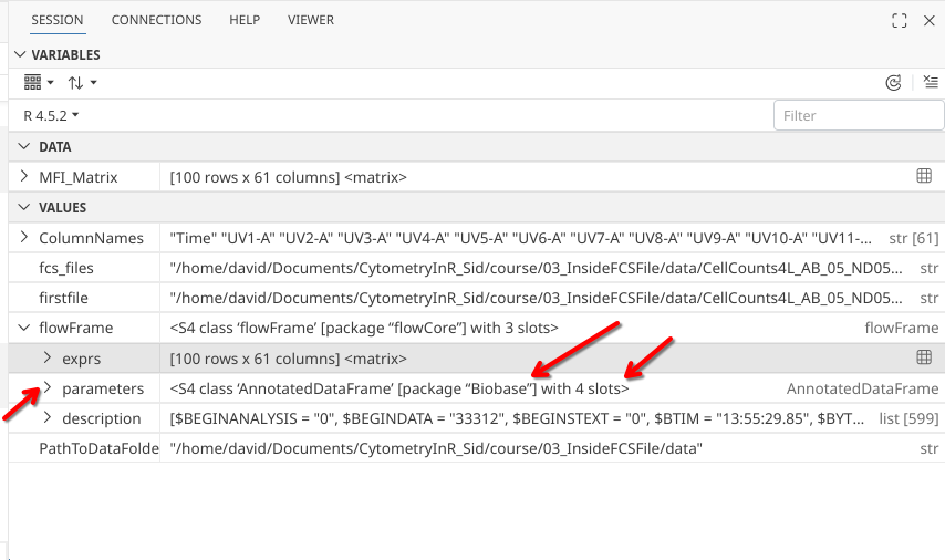
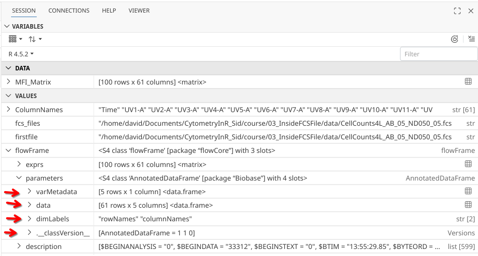
As we look at the next slot in the flowFrame object, we can see that parameters looks like it is going to be another more complex object, as it is showing up as an AnnotatedDataFrame object (defined by the Biobase R package, and itself contains 4 slots).
.
Having carved our way this far into the heart of an .fcs file, we are not about to call it quits now, so CHARGE my fellow cytometrist!!! Click that drop-down arrow!
.
Having survived our charge into the unknown, the four parameter slots appear to be “varMetadata”, “data”, “dimLabels” and “._classVersion_”.
varMetadata
.
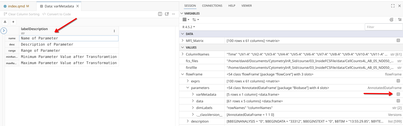
Fortunately for us, both “varMetadata” and “data” at least appear to be table-like objects of a type known as a “data.frame”, so lets click on the grid to open in our editor window.
.
In the case of varMetadata, we seem to have retrieved a column of metadata names.
.
These look reminiscent of what we saw at the top of the read.FCS() column outputs previously
data
.
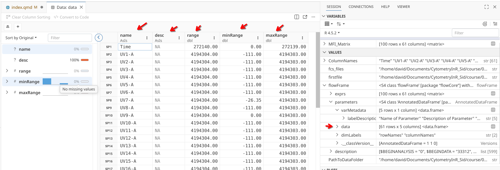
Clicking on the grid for parameters’s data slot will end opening the actual content that was displayed.
.
Let’s try to retrieve the data contained within this slot and save it as it’s own variable/object within our R session. First, we need to open flowFrame object, then use @ to get inside its parameters slot. Since parameters is also a complex object (AnnotatedDataFrame specifically), we will need to use another @ to get inside its data slot:
      name desc   range   minRange maxRange
$P1   Time <NA>  272140    0.00000   272139
$P2  UV1-A <NA> 4194304 -111.00000  4194303
$P3  UV2-A <NA> 4194304 -111.00000  4194303
$P4  UV3-A <NA> 4194304 -111.00000  4194303
$P5  UV4-A <NA> 4194304 -111.00000  4194303
$P6  UV5-A <NA> 4194304 -111.00000  4194303
$P7  UV6-A <NA> 4194304 -111.00000  4194303
$P8  UV7-A <NA> 4194304  -26.34649  4194303
$P9  UV8-A <NA> 4194304 -111.00000  4194303
$P10 UV9-A <NA> 4194304    0.00000  4194303
.
And similarly, we could access with the Bioconductor helper function parameters(), but we would need to specify the accessor for data outside the parenthesis.
.
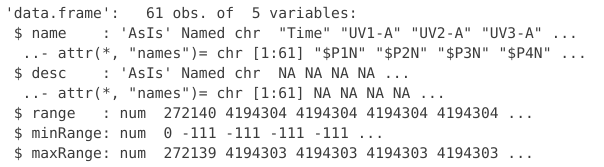
If we ran the str() function, we get the following insight into ParameterData’s object type
'data.frame':   61 obs. of  5 variables:
 $ name    : 'AsIs' Named chr  "Time" "UV1-A" "UV2-A" "UV3-A" ...
  ..- attr(*, "names")= chr [1:61] "$P1N" "$P2N" "$P3N" "$P4N" ...
 $ desc    : 'AsIs' Named chr  NA NA NA NA ...
  ..- attr(*, "names")= chr [1:61] NA NA NA NA ...
 $ range   : num  272140 4194304 4194304 4194304 4194304 ...
 $ minRange: num  0 -111 -111 -111 -111 ...
 $ maxRange: num  272139 4194303 4194303 4194303 4194303 ...
.
We can see this class of object is a “data.frame”. This is one of the more common object types in R, and we will be seeing these extensively throughout the course. We see that each of the columns appears to be designated by a $ followed by the column name, and then type of column (numeric, character, etc).
.
If we are trying to see these columns in R, we notice that data.frame is not like the previous S4 class objets we interacted with, as the @ symbol after doesn’t bring up any suggestions
.
By contrast, adding the $ we saw when using the str() function does retrieve the underlying information
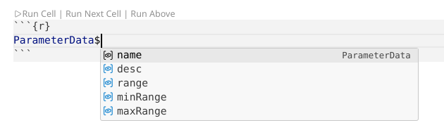
.
As you become more familiar with R, remembering to check what kind of object you are working with, and how to access the contents will with practice become more familiar to you.
.
Similar to what we saw with a matrix, we can subset a data.frame based on the column or row index using square brackets [].
     $P1N      $P2N      $P3N      $P4N      $P5N      $P6N      $P7N      $P8N
   "Time"   "UV1-A"   "UV2-A"   "UV3-A"   "UV4-A"   "UV5-A"   "UV6-A"   "UV7-A"
     $P9N     $P10N     $P11N     $P12N     $P13N     $P14N     $P15N     $P16N
  "UV8-A"   "UV9-A"  "UV10-A"  "UV11-A"  "UV12-A"  "UV13-A"  "UV14-A"  "UV15-A"
    $P17N     $P18N     $P19N     $P20N     $P21N     $P22N     $P23N     $P24N
 "UV16-A"   "SSC-H"   "SSC-A"    "V1-A"    "V2-A"    "V3-A"    "V4-A"    "V5-A"
    $P25N     $P26N     $P27N     $P28N     $P29N     $P30N     $P31N     $P32N
   "V6-A"    "V7-A"    "V8-A"    "V9-A"   "V10-A"   "V11-A"   "V12-A"   "V13-A"
    $P33N     $P34N     $P35N     $P36N     $P37N     $P38N     $P39N     $P40N
  "V14-A"   "V15-A"   "V16-A"   "FSC-H"   "FSC-A" "SSC-B-H" "SSC-B-A"    "B1-A"
    $P41N     $P42N     $P43N     $P44N     $P45N     $P46N     $P47N     $P48N
   "B2-A"    "B3-A"    "B4-A"    "B5-A"    "B6-A"    "B7-A"    "B8-A"    "B9-A"
    $P49N     $P50N     $P51N     $P52N     $P53N     $P54N     $P55N     $P56N
  "B10-A"   "B11-A"   "B12-A"   "B13-A"   "B14-A"    "R1-A"    "R2-A"    "R3-A"
    $P57N     $P58N     $P59N     $P60N     $P61N
   "R4-A"    "R5-A"    "R6-A"    "R7-A"    "R8-A"
.
The individual detectors or fluorophore appear under “name”. For now, based on what we know, the $P# appears to be some sort of name being used as an internal consistent reference to the respective.
.
“desc” is appearing empty for this raw spectral fcs file, but if you were to checked an unmixed file, this would be occupied the marker/ligand name assigned to it during the experiment setup.
.
“range”, “minRange” and “maxRange” are beyond the scope of today, but are used by both instrument manufacturers and software vendors when setting appropiate scaling for a plot. For the actual details, see the Flow Cytometry Standard documentation.
.
Having exhausted our options under parameters “varMetadata” and “data” slots, let’s continue to the next slot.
dimLabels
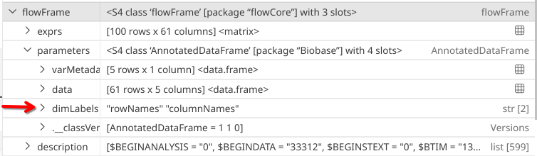
.
In this case, not much is returned. Yey!
classVersion
.
Continuing on to the last slot “.__classVersion__”
.
Also mercifully short, both of these seem to be more involved in defining the S4 class object, and don’t contain anything we need to retrieve today.
Description
.
At this point, we have explored both “exprs” and “parameter” slots for the flowFrame object we created. Let’s tackle the final slot, named description.
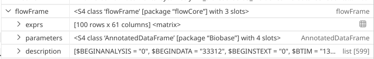
.
When doing so, a very large list is opened within the Positron variables window. While we could scroll through it, it might be easier to retrieve certain number of rows via the console to make interpreting this more structured.
.
To retrieve the list itself, we would need to access the description slot of the flowFrame object. Since it is a slot, we will need to use the @ accessor.
$`$BEGINANALYSIS`
[1] "0"
$`$BEGINDATA`
[1] "33312"
$`$BEGINSTEXT`
[1] "0"
$`$BTIM`
[1] "13:55:29.85"
$`$BYTEORD`
[1] "4,3,2,1"
$`$CYT`
[1] "Aurora"
$`$CYTOLIB_VERSION`
[1] "2.22.0"
$`$CYTSN`
[1] "V0333"
$`$DATATYPE`
[1] "F"
$`$DATE`
[1] "04-Aug-2025"
$`$ENDANALYSIS`
[1] "0"
$`$ENDDATA`
[1] "57711"
$`$ENDSTEXT`
[1] "0"
$`$ETIM`
[1] "13:55:57.02"
$`$FIL`
[1] "CellCounts4L_AB_05-ND050-05.fcs"
$`$INST`
[1] "UMBC"
$`$MODE`
[1] "L"
$`$NEXTDATA`
[1] "0"
$`$OP`
[1] "David Rach"
$`$P10B`
[1] "32"
$`$P10E`
[1] "0,0"
$`$P10N`
[1] "UV9-A"
$`$P10R`
[1] "4194304"
$`$P10TYPE`
[1] "Raw_Fluorescence"
$`$P10V`
[1] "710"
$`$P11B`
[1] "32"
$`$P11E`
[1] "0,0"
$`$P11N`
[1] "UV10-A"
$`$P11R`
[1] "4194304"
$`$P11TYPE`
[1] "Raw_Fluorescence"
$`$P11V`
[1] "377"
$`$P12B`
[1] "32"
$`$P12E`
[1] "0,0"
$`$P12N`
[1] "UV11-A"
$`$P12R`
[1] "4194304"
$`$P12TYPE`
[1] "Raw_Fluorescence"
$`$P12V`
[1] "469"
$`$P13B`
[1] "32"
$`$P13E`
[1] "0,0"
$`$P13N`
[1] "UV12-A"
$`$P13R`
[1] "4194304"
$`$P13TYPE`
[1] "Raw_Fluorescence"
$`$P13V`
[1] "434"
$`$P14B`
[1] "32"
$`$P14E`
[1] "0,0"
$`$P14N`
[1] "UV13-A"
$`$P14R`
[1] "4194304"
$`$P14TYPE`
[1] "Raw_Fluorescence"
$`$P14V`
[1] "564"
$`$P15B`
[1] "32"
$`$P15E`
[1] "0,0"
$`$P15N`
[1] "UV14-A"
$`$P15R`
[1] "4194304"
$`$P15TYPE`
[1] "Raw_Fluorescence"
$`$P15V`
[1] "975"
$`$P16B`
[1] "32"
$`$P16E`
[1] "0,0"
$`$P16N`
[1] "UV15-A"
$`$P16R`
[1] "4194304"
$`$P16TYPE`
[1] "Raw_Fluorescence"
$`$P16V`
[1] "737"
$`$P17B`
[1] "32"
$`$P17E`
[1] "0,0"
$`$P17N`
[1] "UV16-A"
$`$P17R`
[1] "4194304"
$`$P17TYPE`
[1] "Raw_Fluorescence"
$`$P17V`
[1] "1069"
$`$P18B`
[1] "32"
$`$P18E`
[1] "0,0"
$`$P18N`
[1] "SSC-H"
$`$P18R`
[1] "4194304"
$`$P18TYPE`
[1] "Side_Scatter"
$`$P18V`
[1] "334"
$`$P19B`
[1] "32"
$`$P19E`
[1] "0,0"
$`$P19N`
[1] "SSC-A"
$`$P19R`
[1] "4194304"
$`$P19TYPE`
[1] "Side_Scatter"
$`$P19V`
[1] "334"
$`$P1B`
[1] "32"
$`$P1E`
[1] "0,0"
$`$P1N`
[1] "Time"
$`$P1R`
[1] "272140"
$`$P1TYPE`
[1] "Time"
$`$P20B`
[1] "32"
$`$P20E`
[1] "0,0"
$`$P20N`
[1] "V1-A"
$`$P20R`
[1] "4194304"
$`$P20TYPE`
[1] "Raw_Fluorescence"
$`$P20V`
[1] "352"
$`$P21B`
[1] "32"
$`$P21E`
[1] "0,0"
$`$P21N`
[1] "V2-A"
$`$P21R`
[1] "4194304"
$`$P21TYPE`
[1] "Raw_Fluorescence"
$`$P21V`
[1] "412"
$`$P22B`
[1] "32"
$`$P22E`
[1] "0,0"
$`$P22N`
[1] "V3-A"
$`$P22R`
[1] "4194304"
$`$P22TYPE`
[1] "Raw_Fluorescence"
$`$P22V`
[1] "304"
$`$P23B`
[1] "32"
$`$P23E`
[1] "0,0"
$`$P23N`
[1] "V4-A"
$`$P23R`
[1] "4194304"
$`$P23TYPE`
[1] "Raw_Fluorescence"
$`$P23V`
[1] "217"
$`$P24B`
[1] "32"
$`$P24E`
[1] "0,0"
$`$P24N`
[1] "V5-A"
$`$P24R`
[1] "4194304"
$`$P24TYPE`
[1] "Raw_Fluorescence"
$`$P24V`
[1] "257"
$`$P25B`
[1] "32"
$`$P25E`
[1] "0,0"
$`$P25N`
[1] "V6-A"
$`$P25R`
[1] "4194304"
$`$P25TYPE`
[1] "Raw_Fluorescence"
$`$P25V`
[1] "218"
$`$P26B`
[1] "32"
$`$P26E`
[1] "0,0"
$`$P26N`
[1] "V7-A"
$`$P26R`
[1] "4194304"
$`$P26TYPE`
[1] "Raw_Fluorescence"
$`$P26V`
[1] "303"
$`$P27B`
[1] "32"
$`$P27E`
[1] "0,0"
$`$P27N`
[1] "V8-A"
$`$P27R`
[1] "4194304"
$`$P27TYPE`
[1] "Raw_Fluorescence"
$`$P27V`
[1] "461"
$`$P28B`
[1] "32"
$`$P28E`
[1] "0,0"
$`$P28N`
[1] "V9-A"
$`$P28R`
[1] "4194304"
$`$P28TYPE`
[1] "Raw_Fluorescence"
$`$P28V`
[1] "320"
$`$P29B`
[1] "32"
$`$P29E`
[1] "0,0"
$`$P29N`
[1] "V10-A"
$`$P29R`
[1] "4194304"
$`$P29TYPE`
[1] "Raw_Fluorescence"
$`$P29V`
[1] "359"
$`$P2B`
[1] "32"
$`$P2E`
[1] "0,0"
$`$P2N`
[1] "UV1-A"
$`$P2R`
[1] "4194304"
$`$P2TYPE`
[1] "Raw_Fluorescence"
$`$P2V`
[1] "1008"
$`$P30B`
[1] "32"
$`$P30E`
[1] "0,0"
$`$P30N`
[1] "V11-A"
$`$P30R`
[1] "4194304"
$`$P30TYPE`
[1] "Raw_Fluorescence"
$`$P30V`
[1] "271"
$`$P31B`
[1] "32"
$`$P31E`
[1] "0,0"
$`$P31N`
[1] "V12-A"
$`$P31R`
[1] "4194304"
$`$P31TYPE`
[1] "Raw_Fluorescence"
$`$P31V`
[1] "234"
$`$P32B`
[1] "32"
$`$P32E`
[1] "0,0"
$`$P32N`
[1] "V13-A"
$`$P32R`
[1] "4194304"
$`$P32TYPE`
[1] "Raw_Fluorescence"
$`$P32V`
[1] "236"
$`$P33B`
[1] "32"
$`$P33E`
[1] "0,0"
$`$P33N`
[1] "V14-A"
$`$P33R`
[1] "4194304"
$`$P33TYPE`
[1] "Raw_Fluorescence"
$`$P33V`
[1] "318"
$`$P34B`
[1] "32"
$`$P34E`
[1] "0,0"
$`$P34N`
[1] "V15-A"
$`$P34R`
[1] "4194304"
$`$P34TYPE`
[1] "Raw_Fluorescence"
$`$P34V`
[1] "602"
$`$P35B`
[1] "32"
$`$P35E`
[1] "0,0"
$`$P35N`
[1] "V16-A"
$`$P35R`
[1] "4194304"
$`$P35TYPE`
[1] "Raw_Fluorescence"
$`$P35V`
[1] "372"
$`$P36B`
[1] "32"
$`$P36E`
[1] "0,0"
$`$P36N`
[1] "FSC-H"
$`$P36R`
[1] "4194304"
$`$P36TYPE`
[1] "Forward_Scatter"
$`$P36V`
[1] "55"
$`$P37B`
[1] "32"
$`$P37E`
[1] "0,0"
$`$P37N`
[1] "FSC-A"
$`$P37R`
[1] "4194304"
$`$P37TYPE`
[1] "Forward_Scatter"
$`$P37V`
[1] "55"
$`$P38B`
[1] "32"
$`$P38E`
[1] "0,0"
$`$P38N`
[1] "SSC-B-H"
$`$P38R`
[1] "4194304"
$`$P38TYPE`
[1] "Side_Scatter"
$`$P38V`
[1] "241"
$`$P39B`
[1] "32"
$`$P39E`
[1] "0,0"
$`$P39N`
[1] "SSC-B-A"
$`$P39R`
[1] "4194304"
$`$P39TYPE`
[1] "Side_Scatter"
$`$P39V`
[1] "241"
$`$P3B`
[1] "32"
$`$P3E`
[1] "0,0"
$`$P3N`
[1] "UV2-A"
$`$P3R`
[1] "4194304"
$`$P3TYPE`
[1] "Raw_Fluorescence"
$`$P3V`
[1] "286"
$`$P40B`
[1] "32"
$`$P40E`
[1] "0,0"
$`$P40N`
[1] "B1-A"
$`$P40R`
[1] "4194304"
$`$P40TYPE`
[1] "Raw_Fluorescence"
$`$P40V`
[1] "1013"
$`$P41B`
[1] "32"
$`$P41E`
[1] "0,0"
$`$P41N`
[1] "B2-A"
$`$P41R`
[1] "4194304"
$`$P41TYPE`
[1] "Raw_Fluorescence"
$`$P41V`
[1] "483"
$`$P42B`
[1] "32"
$`$P42E`
[1] "0,0"
$`$P42N`
[1] "B3-A"
$`$P42R`
[1] "4194304"
$`$P42TYPE`
[1] "Raw_Fluorescence"
$`$P42V`
[1] "471"
$`$P43B`
[1] "32"
$`$P43E`
[1] "0,0"
$`$P43N`
[1] "B4-A"
$`$P43R`
[1] "4194304"
$`$P43TYPE`
[1] "Raw_Fluorescence"
$`$P43V`
[1] "473"
$`$P44B`
[1] "32"
$`$P44E`
[1] "0,0"
$`$P44N`
[1] "B5-A"
$`$P44R`
[1] "4194304"
$`$P44TYPE`
[1] "Raw_Fluorescence"
$`$P44V`
[1] "467"
$`$P45B`
[1] "32"
$`$P45E`
[1] "0,0"
$`$P45N`
[1] "B6-A"
$`$P45R`
[1] "4194304"
$`$P45TYPE`
[1] "Raw_Fluorescence"
$`$P45V`
[1] "284"
$`$P46B`
[1] "32"
$`$P46E`
[1] "0,0"
$`$P46N`
[1] "B7-A"
$`$P46R`
[1] "4194304"
$`$P46TYPE`
[1] "Raw_Fluorescence"
$`$P46V`
[1] "531"
$`$P47B`
[1] "32"
$`$P47E`
[1] "0,0"
$`$P47N`
[1] "B8-A"
$`$P47R`
[1] "4194304"
$`$P47TYPE`
[1] "Raw_Fluorescence"
$`$P47V`
[1] "432"
$`$P48B`
[1] "32"
$`$P48E`
[1] "0,0"
$`$P48N`
[1] "B9-A"
$`$P48R`
[1] "4194304"
$`$P48TYPE`
[1] "Raw_Fluorescence"
$`$P48V`
[1] "675"
$`$P49B`
[1] "32"
$`$P49E`
[1] "0,0"
$`$P49N`
[1] "B10-A"
$`$P49R`
[1] "4194304"
$`$P49TYPE`
[1] "Raw_Fluorescence"
$`$P49V`
[1] "490"
$`$P4B`
[1] "32"
$`$P4E`
[1] "0,0"
$`$P4N`
[1] "UV3-A"
$`$P4R`
[1] "4194304"
$`$P4TYPE`
[1] "Raw_Fluorescence"
$`$P4V`
[1] "677"
$`$P50B`
[1] "32"
$`$P50E`
[1] "0,0"
$`$P50N`
[1] "B11-A"
$`$P50R`
[1] "4194304"
$`$P50TYPE`
[1] "Raw_Fluorescence"
$`$P50V`
[1] "286"
$`$P51B`
[1] "32"
$`$P51E`
[1] "0,0"
$`$P51N`
[1] "B12-A"
$`$P51R`
[1] "4194304"
$`$P51TYPE`
[1] "Raw_Fluorescence"
$`$P51V`
[1] "407"
$`$P52B`
[1] "32"
$`$P52E`
[1] "0,0"
$`$P52N`
[1] "B13-A"
$`$P52R`
[1] "4194304"
$`$P52TYPE`
[1] "Raw_Fluorescence"
$`$P52V`
[1] "700"
$`$P53B`
[1] "32"
$`$P53E`
[1] "0,0"
$`$P53N`
[1] "B14-A"
$`$P53R`
[1] "4194304"
$`$P53TYPE`
[1] "Raw_Fluorescence"
$`$P53V`
[1] "693"
$`$P54B`
[1] "32"
$`$P54E`
[1] "0,0"
$`$P54N`
[1] "R1-A"
$`$P54R`
[1] "4194304"
$`$P54TYPE`
[1] "Raw_Fluorescence"
$`$P54V`
[1] "158"
$`$P55B`
[1] "32"
$`$P55E`
[1] "0,0"
$`$P55N`
[1] "R2-A"
$`$P55R`
[1] "4194304"
$`$P55TYPE`
[1] "Raw_Fluorescence"
$`$P55V`
[1] "245"
$`$P56B`
[1] "32"
$`$P56E`
[1] "0,0"
$`$P56N`
[1] "R3-A"
$`$P56R`
[1] "4194304"
$`$P56TYPE`
[1] "Raw_Fluorescence"
$`$P56V`
[1] "338"
$`$P57B`
[1] "32"
$`$P57E`
[1] "0,0"
$`$P57N`
[1] "R4-A"
$`$P57R`
[1] "4194304"
$`$P57TYPE`
[1] "Raw_Fluorescence"
$`$P57V`
[1] "238"
$`$P58B`
[1] "32"
$`$P58E`
[1] "0,0"
$`$P58N`
[1] "R5-A"
$`$P58R`
[1] "4194304"
$`$P58TYPE`
[1] "Raw_Fluorescence"
$`$P58V`
[1] "191"
$`$P59B`
[1] "32"
$`$P59E`
[1] "0,0"
$`$P59N`
[1] "R6-A"
$`$P59R`
[1] "4194304"
$`$P59TYPE`
[1] "Raw_Fluorescence"
$`$P59V`
[1] "274"
$`$P5B`
[1] "32"
$`$P5E`
[1] "0,0"
$`$P5N`
[1] "UV4-A"
$`$P5R`
[1] "4194304"
$`$P5TYPE`
[1] "Raw_Fluorescence"
$`$P5V`
[1] "1022"
$`$P60B`
[1] "32"
$`$P60E`
[1] "0,0"
$`$P60N`
[1] "R7-A"
$`$P60R`
[1] "4194304"
$`$P60TYPE`
[1] "Raw_Fluorescence"
$`$P60V`
[1] "524"
$`$P61B`
[1] "32"
$`$P61E`
[1] "0,0"
$`$P61N`
[1] "R8-A"
$`$P61R`
[1] "4194304"
$`$P61TYPE`
[1] "Raw_Fluorescence"
$`$P61V`
[1] "243"
$`$P6B`
[1] "32"
$`$P6E`
[1] "0,0"
$`$P6N`
[1] "UV5-A"
$`$P6R`
[1] "4194304"
$`$P6TYPE`
[1] "Raw_Fluorescence"
$`$P6V`
[1] "616"
$`$P7B`
[1] "32"
$`$P7E`
[1] "0,0"
$`$P7N`
[1] "UV6-A"
$`$P7R`
[1] "4194304"
$`$P7TYPE`
[1] "Raw_Fluorescence"
$`$P7V`
[1] "506"
$`$P8B`
[1] "32"
$`$P8E`
[1] "0,0"
$`$P8N`
[1] "UV7-A"
$`$P8R`
[1] "4194304"
$`$P8TYPE`
[1] "Raw_Fluorescence"
$`$P8V`
[1] "661"
$`$P9B`
[1] "32"
$`$P9E`
[1] "0,0"
$`$P9N`
[1] "UV8-A"
$`$P9R`
[1] "4194304"
$`$P9TYPE`
[1] "Raw_Fluorescence"
$`$P9V`
[1] "514"
$`$PAR`
[1] "61"
$`$PROJ`
[1] "CellCounts4L_AB_05"
$`$SPILLOVER`
UV1-A UV2-A UV3-A UV4-A UV5-A UV6-A UV7-A UV8-A UV9-A UV10-A UV11-A
[1,] 1e+00 0 0 0 0 0 0 0 0 0 0
[2,] 1e-06 1 0 0 0 0 0 0 0 0 0
[3,] 0e+00 0 1 0 0 0 0 0 0 0 0
[4,] 0e+00 0 0 1 0 0 0 0 0 0 0
[5,] 0e+00 0 0 0 1 0 0 0 0 0 0
[6,] 0e+00 0 0 0 0 1 0 0 0 0 0
[7,] 0e+00 0 0 0 0 0 1 0 0 0 0
[8,] 0e+00 0 0 0 0 0 0 1 0 0 0
[9,] 0e+00 0 0 0 0 0 0 0 1 0 0
[10,] 0e+00 0 0 0 0 0 0 0 0 1 0
[11,] 0e+00 0 0 0 0 0 0 0 0 0 1
[12,] 0e+00 0 0 0 0 0 0 0 0 0 0
[13,] 0e+00 0 0 0 0 0 0 0 0 0 0
[14,] 0e+00 0 0 0 0 0 0 0 0 0 0
[15,] 0e+00 0 0 0 0 0 0 0 0 0 0
[16,] 0e+00 0 0 0 0 0 0 0 0 0 0
[17,] 0e+00 0 0 0 0 0 0 0 0 0 0
[18,] 0e+00 0 0 0 0 0 0 0 0 0 0
[19,] 0e+00 0 0 0 0 0 0 0 0 0 0
[20,] 0e+00 0 0 0 0 0 0 0 0 0 0
[21,] 0e+00 0 0 0 0 0 0 0 0 0 0
[22,] 0e+00 0 0 0 0 0 0 0 0 0 0
[23,] 0e+00 0 0 0 0 0 0 0 0 0 0
[24,] 0e+00 0 0 0 0 0 0 0 0 0 0
[25,] 0e+00 0 0 0 0 0 0 0 0 0 0
[26,] 0e+00 0 0 0 0 0 0 0 0 0 0
[27,] 0e+00 0 0 0 0 0 0 0 0 0 0
[28,] 0e+00 0 0 0 0 0 0 0 0 0 0
[29,] 0e+00 0 0 0 0 0 0 0 0 0 0
[30,] 0e+00 0 0 0 0 0 0 0 0 0 0
[31,] 0e+00 0 0 0 0 0 0 0 0 0 0
[32,] 0e+00 0 0 0 0 0 0 0 0 0 0
[33,] 0e+00 0 0 0 0 0 0 0 0 0 0
[34,] 0e+00 0 0 0 0 0 0 0 0 0 0
[35,] 0e+00 0 0 0 0 0 0 0 0 0 0
[36,] 0e+00 0 0 0 0 0 0 0 0 0 0
[37,] 0e+00 0 0 0 0 0 0 0 0 0 0
[38,] 0e+00 0 0 0 0 0 0 0 0 0 0
[39,] 0e+00 0 0 0 0 0 0 0 0 0 0
[40,] 0e+00 0 0 0 0 0 0 0 0 0 0
[41,] 0e+00 0 0 0 0 0 0 0 0 0 0
[42,] 0e+00 0 0 0 0 0 0 0 0 0 0
[43,] 0e+00 0 0 0 0 0 0 0 0 0 0
[44,] 0e+00 0 0 0 0 0 0 0 0 0 0
[45,] 0e+00 0 0 0 0 0 0 0 0 0 0
[46,] 0e+00 0 0 0 0 0 0 0 0 0 0
[47,] 0e+00 0 0 0 0 0 0 0 0 0 0
[48,] 0e+00 0 0 0 0 0 0 0 0 0 0
[49,] 0e+00 0 0 0 0 0 0 0 0 0 0
[50,] 0e+00 0 0 0 0 0 0 0 0 0 0
[51,] 0e+00 0 0 0 0 0 0 0 0 0 0
[52,] 0e+00 0 0 0 0 0 0 0 0 0 0
[53,] 0e+00 0 0 0 0 0 0 0 0 0 0
[54,] 0e+00 0 0 0 0 0 0 0 0 0 0
UV12-A UV13-A UV14-A UV15-A UV16-A V1-A V2-A V3-A V4-A V5-A V6-A V7-A
[1,] 0 0 0 0 0 0 0 0 0 0 0 0
[2,] 0 0 0 0 0 0 0 0 0 0 0 0
[3,] 0 0 0 0 0 0 0 0 0 0 0 0
[4,] 0 0 0 0 0 0 0 0 0 0 0 0
[5,] 0 0 0 0 0 0 0 0 0 0 0 0
[6,] 0 0 0 0 0 0 0 0 0 0 0 0
[7,] 0 0 0 0 0 0 0 0 0 0 0 0
[8,] 0 0 0 0 0 0 0 0 0 0 0 0
[9,] 0 0 0 0 0 0 0 0 0 0 0 0
[10,] 0 0 0 0 0 0 0 0 0 0 0 0
[11,] 0 0 0 0 0 0 0 0 0 0 0 0
[12,] 1 0 0 0 0 0 0 0 0 0 0 0
[13,] 0 1 0 0 0 0 0 0 0 0 0 0
[14,] 0 0 1 0 0 0 0 0 0 0 0 0
[15,] 0 0 0 1 0 0 0 0 0 0 0 0
[16,] 0 0 0 0 1 0 0 0 0 0 0 0
[17,] 0 0 0 0 0 1 0 0 0 0 0 0
[18,] 0 0 0 0 0 0 1 0 0 0 0 0
[19,] 0 0 0 0 0 0 0 1 0 0 0 0
[20,] 0 0 0 0 0 0 0 0 1 0 0 0
[21,] 0 0 0 0 0 0 0 0 0 1 0 0
[22,] 0 0 0 0 0 0 0 0 0 0 1 0
[23,] 0 0 0 0 0 0 0 0 0 0 0 1
[24,] 0 0 0 0 0 0 0 0 0 0 0 0
[25,] 0 0 0 0 0 0 0 0 0 0 0 0
[26,] 0 0 0 0 0 0 0 0 0 0 0 0
[27,] 0 0 0 0 0 0 0 0 0 0 0 0
[28,] 0 0 0 0 0 0 0 0 0 0 0 0
[29,] 0 0 0 0 0 0 0 0 0 0 0 0
[30,] 0 0 0 0 0 0 0 0 0 0 0 0
[31,] 0 0 0 0 0 0 0 0 0 0 0 0
[32,] 0 0 0 0 0 0 0 0 0 0 0 0
[33,] 0 0 0 0 0 0 0 0 0 0 0 0
[34,] 0 0 0 0 0 0 0 0 0 0 0 0
[35,] 0 0 0 0 0 0 0 0 0 0 0 0
[36,] 0 0 0 0 0 0 0 0 0 0 0 0
[37,] 0 0 0 0 0 0 0 0 0 0 0 0
[38,] 0 0 0 0 0 0 0 0 0 0 0 0
[39,] 0 0 0 0 0 0 0 0 0 0 0 0
[40,] 0 0 0 0 0 0 0 0 0 0 0 0
[41,] 0 0 0 0 0 0 0 0 0 0 0 0
[42,] 0 0 0 0 0 0 0 0 0 0 0 0
[43,] 0 0 0 0 0 0 0 0 0 0 0 0
[44,] 0 0 0 0 0 0 0 0 0 0 0 0
[45,] 0 0 0 0 0 0 0 0 0 0 0 0
[46,] 0 0 0 0 0 0 0 0 0 0 0 0
[47,] 0 0 0 0 0 0 0 0 0 0 0 0
[48,] 0 0 0 0 0 0 0 0 0 0 0 0
[49,] 0 0 0 0 0 0 0 0 0 0 0 0
[50,] 0 0 0 0 0 0 0 0 0 0 0 0
[51,] 0 0 0 0 0 0 0 0 0 0 0 0
[52,] 0 0 0 0 0 0 0 0 0 0 0 0
[53,] 0 0 0 0 0 0 0 0 0 0 0 0
[54,] 0 0 0 0 0 0 0 0 0 0 0 0
V8-A V9-A V10-A V11-A V12-A V13-A V14-A V15-A V16-A B1-A B2-A B3-A B4-A
[1,] 0 0 0 0 0 0 0 0 0 0 0 0 0
[2,] 0 0 0 0 0 0 0 0 0 0 0 0 0
[3,] 0 0 0 0 0 0 0 0 0 0 0 0 0
[4,] 0 0 0 0 0 0 0 0 0 0 0 0 0
[5,] 0 0 0 0 0 0 0 0 0 0 0 0 0
[6,] 0 0 0 0 0 0 0 0 0 0 0 0 0
[7,] 0 0 0 0 0 0 0 0 0 0 0 0 0
[8,] 0 0 0 0 0 0 0 0 0 0 0 0 0
[9,] 0 0 0 0 0 0 0 0 0 0 0 0 0
[10,] 0 0 0 0 0 0 0 0 0 0 0 0 0
[11,] 0 0 0 0 0 0 0 0 0 0 0 0 0
[12,] 0 0 0 0 0 0 0 0 0 0 0 0 0
[13,] 0 0 0 0 0 0 0 0 0 0 0 0 0
[14,] 0 0 0 0 0 0 0 0 0 0 0 0 0
[15,] 0 0 0 0 0 0 0 0 0 0 0 0 0
[16,] 0 0 0 0 0 0 0 0 0 0 0 0 0
[17,] 0 0 0 0 0 0 0 0 0 0 0 0 0
[18,] 0 0 0 0 0 0 0 0 0 0 0 0 0
[19,] 0 0 0 0 0 0 0 0 0 0 0 0 0
[20,] 0 0 0 0 0 0 0 0 0 0 0 0 0
[21,] 0 0 0 0 0 0 0 0 0 0 0 0 0
[22,] 0 0 0 0 0 0 0 0 0 0 0 0 0
[23,] 0 0 0 0 0 0 0 0 0 0 0 0 0
[24,] 1 0 0 0 0 0 0 0 0 0 0 0 0
[25,] 0 1 0 0 0 0 0 0 0 0 0 0 0
[26,] 0 0 1 0 0 0 0 0 0 0 0 0 0
[27,] 0 0 0 1 0 0 0 0 0 0 0 0 0
[28,] 0 0 0 0 1 0 0 0 0 0 0 0 0
[29,] 0 0 0 0 0 1 0 0 0 0 0 0 0
[30,] 0 0 0 0 0 0 1 0 0 0 0 0 0
[31,] 0 0 0 0 0 0 0 1 0 0 0 0 0
[32,] 0 0 0 0 0 0 0 0 1 0 0 0 0
[33,] 0 0 0 0 0 0 0 0 0 1 0 0 0
[34,] 0 0 0 0 0 0 0 0 0 0 1 0 0
[35,] 0 0 0 0 0 0 0 0 0 0 0 1 0
[36,] 0 0 0 0 0 0 0 0 0 0 0 0 1
[37,] 0 0 0 0 0 0 0 0 0 0 0 0 0
[38,] 0 0 0 0 0 0 0 0 0 0 0 0 0
[39,] 0 0 0 0 0 0 0 0 0 0 0 0 0
[40,] 0 0 0 0 0 0 0 0 0 0 0 0 0
[41,] 0 0 0 0 0 0 0 0 0 0 0 0 0
[42,] 0 0 0 0 0 0 0 0 0 0 0 0 0
[43,] 0 0 0 0 0 0 0 0 0 0 0 0 0
[44,] 0 0 0 0 0 0 0 0 0 0 0 0 0
[45,] 0 0 0 0 0 0 0 0 0 0 0 0 0
[46,] 0 0 0 0 0 0 0 0 0 0 0 0 0
[47,] 0 0 0 0 0 0 0 0 0 0 0 0 0
[48,] 0 0 0 0 0 0 0 0 0 0 0 0 0
[49,] 0 0 0 0 0 0 0 0 0 0 0 0 0
[50,] 0 0 0 0 0 0 0 0 0 0 0 0 0
[51,] 0 0 0 0 0 0 0 0 0 0 0 0 0
[52,] 0 0 0 0 0 0 0 0 0 0 0 0 0
[53,] 0 0 0 0 0 0 0 0 0 0 0 0 0
[54,] 0 0 0 0 0 0 0 0 0 0 0 0 0
B5-A B6-A B7-A B8-A B9-A B10-A B11-A B12-A B13-A B14-A R1-A R2-A R3-A
[1,] 0 0 0 0 0 0 0 0 0 0 0 0 0
[2,] 0 0 0 0 0 0 0 0 0 0 0 0 0
[3,] 0 0 0 0 0 0 0 0 0 0 0 0 0
[4,] 0 0 0 0 0 0 0 0 0 0 0 0 0
[5,] 0 0 0 0 0 0 0 0 0 0 0 0 0
[6,] 0 0 0 0 0 0 0 0 0 0 0 0 0
[7,] 0 0 0 0 0 0 0 0 0 0 0 0 0
[8,] 0 0 0 0 0 0 0 0 0 0 0 0 0
[9,] 0 0 0 0 0 0 0 0 0 0 0 0 0
[10,] 0 0 0 0 0 0 0 0 0 0 0 0 0
[11,] 0 0 0 0 0 0 0 0 0 0 0 0 0
[12,] 0 0 0 0 0 0 0 0 0 0 0 0 0
[13,] 0 0 0 0 0 0 0 0 0 0 0 0 0
[14,] 0 0 0 0 0 0 0 0 0 0 0 0 0
[15,] 0 0 0 0 0 0 0 0 0 0 0 0 0
[16,] 0 0 0 0 0 0 0 0 0 0 0 0 0
[17,] 0 0 0 0 0 0 0 0 0 0 0 0 0
[18,] 0 0 0 0 0 0 0 0 0 0 0 0 0
[19,] 0 0 0 0 0 0 0 0 0 0 0 0 0
[20,] 0 0 0 0 0 0 0 0 0 0 0 0 0
[21,] 0 0 0 0 0 0 0 0 0 0 0 0 0
[22,] 0 0 0 0 0 0 0 0 0 0 0 0 0
[23,] 0 0 0 0 0 0 0 0 0 0 0 0 0
[24,] 0 0 0 0 0 0 0 0 0 0 0 0 0
[25,] 0 0 0 0 0 0 0 0 0 0 0 0 0
[26,] 0 0 0 0 0 0 0 0 0 0 0 0 0
[27,] 0 0 0 0 0 0 0 0 0 0 0 0 0
[28,] 0 0 0 0 0 0 0 0 0 0 0 0 0
[29,] 0 0 0 0 0 0 0 0 0 0 0 0 0
[30,] 0 0 0 0 0 0 0 0 0 0 0 0 0
[31,] 0 0 0 0 0 0 0 0 0 0 0 0 0
[32,] 0 0 0 0 0 0 0 0 0 0 0 0 0
[33,] 0 0 0 0 0 0 0 0 0 0 0 0 0
[34,] 0 0 0 0 0 0 0 0 0 0 0 0 0
[35,] 0 0 0 0 0 0 0 0 0 0 0 0 0
[36,] 0 0 0 0 0 0 0 0 0 0 0 0 0
[37,] 1 0 0 0 0 0 0 0 0 0 0 0 0
[38,] 0 1 0 0 0 0 0 0 0 0 0 0 0
[39,] 0 0 1 0 0 0 0 0 0 0 0 0 0
[40,] 0 0 0 1 0 0 0 0 0 0 0 0 0
[41,] 0 0 0 0 1 0 0 0 0 0 0 0 0
[42,] 0 0 0 0 0 1 0 0 0 0 0 0 0
[43,] 0 0 0 0 0 0 1 0 0 0 0 0 0
[44,] 0 0 0 0 0 0 0 1 0 0 0 0 0
[45,] 0 0 0 0 0 0 0 0 1 0 0 0 0
[46,] 0 0 0 0 0 0 0 0 0 1 0 0 0
[47,] 0 0 0 0 0 0 0 0 0 0 1 0 0
[48,] 0 0 0 0 0 0 0 0 0 0 0 1 0
[49,] 0 0 0 0 0 0 0 0 0 0 0 0 1
[50,] 0 0 0 0 0 0 0 0 0 0 0 0 0
[51,] 0 0 0 0 0 0 0 0 0 0 0 0 0
[52,] 0 0 0 0 0 0 0 0 0 0 0 0 0
[53,] 0 0 0 0 0 0 0 0 0 0 0 0 0
[54,] 0 0 0 0 0 0 0 0 0 0 0 0 0
R4-A R5-A R6-A R7-A R8-A
[1,] 0 0 0 0 0
[2,] 0 0 0 0 0
[3,] 0 0 0 0 0
[4,] 0 0 0 0 0
[5,] 0 0 0 0 0
[6,] 0 0 0 0 0
[7,] 0 0 0 0 0
[8,] 0 0 0 0 0
[9,] 0 0 0 0 0
[10,] 0 0 0 0 0
[11,] 0 0 0 0 0
[12,] 0 0 0 0 0
[13,] 0 0 0 0 0
[14,] 0 0 0 0 0
[15,] 0 0 0 0 0
[16,] 0 0 0 0 0
[17,] 0 0 0 0 0
[18,] 0 0 0 0 0
[19,] 0 0 0 0 0
[20,] 0 0 0 0 0
[21,] 0 0 0 0 0
[22,] 0 0 0 0 0
[23,] 0 0 0 0 0
[24,] 0 0 0 0 0
[25,] 0 0 0 0 0
[26,] 0 0 0 0 0
[27,] 0 0 0 0 0
[28,] 0 0 0 0 0
[29,] 0 0 0 0 0
[30,] 0 0 0 0 0
[31,] 0 0 0 0 0
[32,] 0 0 0 0 0
[33,] 0 0 0 0 0
[34,] 0 0 0 0 0
[35,] 0 0 0 0 0
[36,] 0 0 0 0 0
[37,] 0 0 0 0 0
[38,] 0 0 0 0 0
[39,] 0 0 0 0 0
[40,] 0 0 0 0 0
[41,] 0 0 0 0 0
[42,] 0 0 0 0 0
[43,] 0 0 0 0 0
[44,] 0 0 0 0 0
[45,] 0 0 0 0 0
[46,] 0 0 0 0 0
[47,] 0 0 0 0 0
[48,] 0 0 0 0 0
[49,] 0 0 0 0 0
[50,] 1 0 0 0 0
[51,] 0 1 0 0 0
[52,] 0 0 1 0 0
[53,] 0 0 0 1 0
[54,] 0 0 0 0 1
$`$TIMESTEP`
[1] "0.0001"
$`$TOT`
[1] "100"
$`$VOL`
[1] "30.31"
$`APPLY COMPENSATION`
[1] "FALSE"
$CHARSET
[1] "utf-8"
$CREATOR
[1] "SpectroFlo 3.3.0"
$FCSversion
[1] "3"
$FILENAME
[1] "data/CellCounts4L_AB_05_ND050_05.fcs"
$`FSC ASF`
[1] "1.21"
$GROUPNAME
[1] "ND050"
$GUID
[1] "CellCounts4L_AB_05-ND050-05.fcs"
$LASER1ASF
[1] "1.09"
$LASER1DELAY
[1] "-19.525"
$LASER1NAME
[1] "Violet"
$LASER2ASF
[1] "1.14"
$LASER2DELAY
[1] "0"
$LASER2NAME
[1] "Blue"
$LASER3ASF
[1] "1.02"
$LASER3DELAY
[1] "20.15"
$LASER3NAME
[1] "Red"
$LASER4ASF
[1] "0.92"
$LASER4DELAY
[1] "40.725"
$LASER4NAME
[1] "UV"
$ORIGINALGUID
[1] "CellCounts4L_AB_05-ND050-05.fcs"
$P10DISPLAY
[1] "LOG"
$P11DISPLAY
[1] "LOG"
$P12DISPLAY
[1] "LOG"
$P13DISPLAY
[1] "LOG"
$P14DISPLAY
[1] "LOG"
$P15DISPLAY
[1] "LOG"
$P16DISPLAY
[1] "LOG"
$P17DISPLAY
[1] "LOG"
$P18DISPLAY
[1] "LIN"
$P19DISPLAY
[1] "LIN"
$P1DISPLAY
[1] "LOG"
$P20DISPLAY
[1] "LOG"
$P21DISPLAY
[1] "LOG"
$P22DISPLAY
[1] "LOG"
$P23DISPLAY
[1] "LOG"
$P24DISPLAY
[1] "LOG"
$P25DISPLAY
[1] "LOG"
$P26DISPLAY
[1] "LOG"
$P27DISPLAY
[1] "LOG"
$P28DISPLAY
[1] "LOG"
$P29DISPLAY
[1] "LOG"
$P2DISPLAY
[1] "LOG"
$P30DISPLAY
[1] "LOG"
$P31DISPLAY
[1] "LOG"
$P32DISPLAY
[1] "LOG"
$P33DISPLAY
[1] "LOG"
$P34DISPLAY
[1] "LOG"
$P35DISPLAY
[1] "LOG"
$P36DISPLAY
[1] "LIN"
$P37DISPLAY
[1] "LIN"
$P38DISPLAY
[1] "LIN"
$P39DISPLAY
[1] "LIN"
$P3DISPLAY
[1] "LOG"
$P40DISPLAY
[1] "LOG"
$P41DISPLAY
[1] "LOG"
$P42DISPLAY
[1] "LOG"
$P43DISPLAY
[1] "LOG"
$P44DISPLAY
[1] "LOG"
$P45DISPLAY
[1] "LOG"
$P46DISPLAY
[1] "LOG"
$P47DISPLAY
[1] "LOG"
$P48DISPLAY
[1] "LOG"
$P49DISPLAY
[1] "LOG"
$P4DISPLAY
[1] "LOG"
$P50DISPLAY
[1] "LOG"
$P51DISPLAY
[1] "LOG"
$P52DISPLAY
[1] "LOG"
$P53DISPLAY
[1] "LOG"
$P54DISPLAY
[1] "LOG"
$P55DISPLAY
[1] "LOG"
$P56DISPLAY
[1] "LOG"
$P57DISPLAY
[1] "LOG"
$P58DISPLAY
[1] "LOG"
$P59DISPLAY
[1] "LOG"
$P5DISPLAY
[1] "LOG"
$P60DISPLAY
[1] "LOG"
$P61DISPLAY
[1] "LOG"
$P6DISPLAY
[1] "LOG"
$P7DISPLAY
[1] "LOG"
$P8DISPLAY
[1] "LOG"
$P9DISPLAY
[1] "LOG"
$THRESHOLD
[1] "(FSC,50000)"
$TUBENAME
[1] "05"
$USERSETTINGNAME
[1] "DTR_CellCounts"
$`WINDOW EXTENSION`
[1] "3".
The returned list is a little too large to reasonably explore. We can attempt to subset using the head() function as shown below
.
Alternatively, it might be better to subset based on position index
.
And just as we saw for exprs and parameters, there is also a Bioconductor helper keyword() function to access this same information directly from the flowFrame.
.
If we run the class() function, we can see that DescriptionList is an actual “list”.
.
This is in contrast to the vectors we have previously generated. While these are also list like, they are what are known as as atomic list, which contain values that are all either characters, numerics or logicals.
.
A list on the other hand is not restricted to contain objects composed entirely of a certain atomic type. For example, I could include the three previous vectors into a list using the list() function.
.
We can see that with the Description/Keyword list we retrieved from our flowFrame shares a somewhat similar format.
.
But in this case, there are also names present ($BEGINANALYSIS, $BEGINDATA, etc). What if we had tried to provide names to our List of Vectors? Would the format match?
.
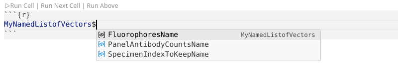
When we assigned a name to each of the vectors (by providing an equal to = ), we get the same kind of structure format to what we see in Description.
List of 3
$ FluorophoresNamed : chr [1:4] "BV421" "FITC" "PE" "APC"
$ PanelAntibodyCountsNamed: num [1:7] 5 12 19 26 34 46 51
$ SpecimenIndexToKeepNamed: logi [1:4] TRUE TRUE FALSE TRUE.
We could then subsequently be able to isolate items from that list using the $ operator.
.
Alternatively, we could also access by list index position
.
Remembering back to the original output from read.FCS() we remember that it mentioned 599 keywords being in the description slot, so now we know that this is what was being referenced.
Keyword Madness
.
Rather than go through the keywords individually (in which case we would be here through tomorrow), let’s take a birds eye view of the contents of this list.
$`$BEGINANALYSIS`
[1] "0"

$`$BEGINDATA`
[1] "33312"

$`$BEGINSTEXT`
[1] "0"

$`$BTIM`
[1] "13:55:29.85"

$`$BYTEORD`
[1] "4,3,2,1"
$`$CYT`
[1] "Aurora"
$`$CYTOLIB_VERSION`
[1] "2.22.0"
$`$CYTSN`
[1] "V0333"
$`$DATATYPE`
[1] "F"
$`$DATE`
[1] "04-Aug-2025"
$`$ENDANALYSIS`
[1] "0"
$`$ENDDATA`
[1] "57711"
$`$ENDSTEXT`
[1] "0"
$`$ETIM`
[1] "13:55:57.02"
$`$FIL`
[1] "CellCounts4L_AB_05-ND050-05.fcs"
$`$INST`
[1] "UMBC"
$`$MODE`
[1] "L"
$`$NEXTDATA`
[1] "0"Early Metadata
.
Within the initial portion, we are getting back metadata keywords related to where and how the particular file was acquired. Keywords of potential interest include:
Start Time
What time was the .fcs file acquired
Cytometer
What type of cytometer was the .fcs file acquired on
Cytometer Serial Number
Manufacturer Serial Number of the Cytometer
FCS File Acquisition Date
What was the date of acquisition
Acquisition End Time
What time was acquisition stopped
File Name
Name of the .fcs file
Operator
Who acquired the .fcs file
Detector Values
.
The next major stretch of keywords encode parameter values associated with the individual detectors for at the time of acquisition.
$`$P10B`
[1] "32"

$`$P10E`
[1] "0,0"

$`$P10N`
[1] "UV9-A"

$`$P10R`
[1] "4194304"

$`$P10TYPE`
[1] "Raw_Fluorescence"

$`$P10V`
[1] "710"

$`$P11B`
[1] "32"

$`$P11E`
[1] "0,0"

$`$P11N`
[1] "UV10-A"

$`$P11R`
[1] "4194304"

$`$P11TYPE`
[1] "Raw_Fluorescence"

$`$P11V`
[1] "377"

$`$P12B`
[1] "32"

$`$P12E`
[1] "0,0"

$`$P12N`
[1] "UV11-A"

$`$P12R`
[1] "4194304"

$`$P12TYPE`
[1] "Raw_Fluorescence"

$`$P12V`
[1] "469"

$`$P13B`
[1] "32"

$`$P13E`
[1] "0,0"

$`$P13N`
[1] "UV12-A"

$`$P13R`
[1] "4194304"

$`$P13TYPE`
[1] "Raw_Fluorescence"

$`$P13V`
[1] "434"

$`$P14B`
[1] "32"

$`$P14E`
[1] "0,0"

$`$P14N`
[1] "UV13-A"

$`$P14R`
[1] "4194304"

$`$P14TYPE`
[1] "Raw_Fluorescence"

$`$P14V`
[1] "564"

$`$P15B`
[1] "32"

$`$P15E`
[1] "0,0"

$`$P15N`
[1] "UV14-A"

$`$P15R`
[1] "4194304"

$`$P15TYPE`
[1] "Raw_Fluorescence"

$`$P15V`
[1] "975"

$`$P16B`
[1] "32"

$`$P16E`
[1] "0,0"

$`$P16N`
[1] "UV15-A"

$`$P16R`
[1] "4194304"

$`$P16TYPE`
[1] "Raw_Fluorescence"

$`$P16V`
[1] "737"

$`$P17B`
[1] "32"

$`$P17E`
[1] "0,0"

$`$P17N`
[1] "UV16-A"

$`$P17R`
[1] "4194304"

$`$P17TYPE`
[1] "Raw_Fluorescence"

$`$P17V`
[1] "1069"

$`$P18B`
[1] "32"

$`$P18E`
[1] "0,0"

$`$P18N`
[1] "SSC-H"

$`$P18R`
[1] "4194304"

$`$P18TYPE`
[1] "Side_Scatter"

$`$P18V`
[1] "334"

$`$P19B`
[1] "32"

$`$P19E`
[1] "0,0"

$`$P19N`
[1] "SSC-A"

$`$P19R`
[1] "4194304"

$`$P19TYPE`
[1] "Side_Scatter"

$`$P19V`
[1] "334"

$`$P1B`
[1] "32"

$`$P1E`
[1] "0,0"

$`$P1N`
[1] "Time"

$`$P1R`
[1] "272140"

$`$P1TYPE`
[1] "Time"

$`$P20B`
[1] "32"

$`$P20E`
[1] "0,0"

$`$P20N`
[1] "V1-A"

$`$P20R`
[1] "4194304"

$`$P20TYPE`
[1] "Raw_Fluorescence"

$`$P20V`
[1] "352"

$`$P21B`
[1] "32"

$`$P21E`
[1] "0,0"

$`$P21N`
[1] "V2-A"

$`$P21R`
[1] "4194304"

$`$P21TYPE`
[1] "Raw_Fluorescence"

$`$P21V`
[1] "412"

$`$P22B`
[1] "32"

$`$P22E`
[1] "0,0"

$`$P22N`
[1] "V3-A"

$`$P22R`
[1] "4194304"

$`$P22TYPE`
[1] "Raw_Fluorescence"

$`$P22V`
[1] "304"

$`$P23B`
[1] "32"

$`$P23E`
[1] "0,0"

$`$P23N`
[1] "V4-A"

$`$P23R`
[1] "4194304"

$`$P23TYPE`
[1] "Raw_Fluorescence"

$`$P23V`
[1] "217"

$`$P24B`
[1] "32"

$`$P24E`
[1] "0,0"

$`$P24N`
[1] "V5-A"

$`$P24R`
[1] "4194304"

$`$P24TYPE`
[1] "Raw_Fluorescence"

$`$P24V`
[1] "257"

$`$P25B`
[1] "32"

$`$P25E`
[1] "0,0"

$`$P25N`
[1] "V6-A"

$`$P25R`
[1] "4194304"

$`$P25TYPE`
[1] "Raw_Fluorescence"

$`$P25V`
[1] "218"

$`$P26B`
[1] "32"

$`$P26E`
[1] "0,0"

$`$P26N`
[1] "V7-A"

$`$P26R`
[1] "4194304"

$`$P26TYPE`
[1] "Raw_Fluorescence"

$`$P26V`
[1] "303"

$`$P27B`
[1] "32"

$`$P27E`
[1] "0,0"

$`$P27N`
[1] "V8-A"

$`$P27R`
[1] "4194304"

$`$P27TYPE`
[1] "Raw_Fluorescence"

$`$P27V`
[1] "461"

$`$P28B`
[1] "32"

$`$P28E`
[1] "0,0"

$`$P28N`
[1] "V9-A"

$`$P28R`
[1] "4194304"

$`$P28TYPE`
[1] "Raw_Fluorescence"

$`$P28V`
[1] "320"

$`$P29B`
[1] "32"

$`$P29E`
[1] "0,0"

$`$P29N`
[1] "V10-A"

$`$P29R`
[1] "4194304"

$`$P29TYPE`
[1] "Raw_Fluorescence"

$`$P29V`
[1] "359"

$`$P2B`
[1] "32"

$`$P2E`
[1] "0,0"

$`$P2N`
[1] "UV1-A"

$`$P2R`
[1] "4194304"

$`$P2TYPE`
[1] "Raw_Fluorescence"

$`$P2V`
[1] "1008"

$`$P30B`
[1] "32"

$`$P30E`
[1] "0,0"

$`$P30N`
[1] "V11-A"

$`$P30R`
[1] "4194304"

$`$P30TYPE`
[1] "Raw_Fluorescence"

$`$P30V`
[1] "271"

$`$P31B`
[1] "32"

$`$P31E`
[1] "0,0"

$`$P31N`
[1] "V12-A"

$`$P31R`
[1] "4194304"

$`$P31TYPE`
[1] "Raw_Fluorescence"

$`$P31V`
[1] "234"

$`$P32B`
[1] "32"

$`$P32E`
[1] "0,0"

$`$P32N`
[1] "V13-A"

$`$P32R`
[1] "4194304"

$`$P32TYPE`
[1] "Raw_Fluorescence"

$`$P32V`
[1] "236"

$`$P33B`
[1] "32"

$`$P33E`
[1] "0,0"

$`$P33N`
[1] "V14-A"

$`$P33R`
[1] "4194304"

$`$P33TYPE`
[1] "Raw_Fluorescence"

$`$P33V`
[1] "318"

$`$P34B`
[1] "32"

$`$P34E`
[1] "0,0"

$`$P34N`
[1] "V15-A"

$`$P34R`
[1] "4194304"

$`$P34TYPE`
[1] "Raw_Fluorescence"

$`$P34V`
[1] "602"

$`$P35B`
[1] "32"

$`$P35E`
[1] "0,0"

$`$P35N`
[1] "V16-A"

$`$P35R`
[1] "4194304"

$`$P35TYPE`
[1] "Raw_Fluorescence"

$`$P35V`
[1] "372"

$`$P36B`
[1] "32"

$`$P36E`
[1] "0,0"

$`$P36N`
[1] "FSC-H"

$`$P36R`
[1] "4194304"

$`$P36TYPE`
[1] "Forward_Scatter"

$`$P36V`
[1] "55"

$`$P37B`
[1] "32"

$`$P37E`
[1] "0,0"

$`$P37N`
[1] "FSC-A"

$`$P37R`
[1] "4194304"

$`$P37TYPE`
[1] "Forward_Scatter"

$`$P37V`
[1] "55"

$`$P38B`
[1] "32"

$`$P38E`
[1] "0,0"

$`$P38N`
[1] "SSC-B-H"

$`$P38R`
[1] "4194304"

$`$P38TYPE`
[1] "Side_Scatter"

$`$P38V`
[1] "241"

$`$P39B`
[1] "32"

$`$P39E`
[1] "0,0"

$`$P39N`
[1] "SSC-B-A"

$`$P39R`
[1] "4194304"

$`$P39TYPE`
[1] "Side_Scatter"

$`$P39V`
[1] "241"

$`$P3B`
[1] "32"

$`$P3E`
[1] "0,0"

$`$P3N`
[1] "UV2-A"

$`$P3R`
[1] "4194304"

$`$P3TYPE`
[1] "Raw_Fluorescence"

$`$P3V`
[1] "286"

$`$P40B`
[1] "32"

$`$P40E`
[1] "0,0"

$`$P40N`
[1] "B1-A"

$`$P40R`
[1] "4194304"

$`$P40TYPE`
[1] "Raw_Fluorescence"

$`$P40V`
[1] "1013"

$`$P41B`
[1] "32"

$`$P41E`
[1] "0,0"

$`$P41N`
[1] "B2-A"

$`$P41R`
[1] "4194304"

$`$P41TYPE`
[1] "Raw_Fluorescence"

$`$P41V`
[1] "483"

$`$P42B`
[1] "32"

$`$P42E`
[1] "0,0"

$`$P42N`
[1] "B3-A"

$`$P42R`
[1] "4194304"

$`$P42TYPE`
[1] "Raw_Fluorescence"

$`$P42V`
[1] "471"

$`$P43B`
[1] "32"

$`$P43E`
[1] "0,0"

$`$P43N`
[1] "B4-A"

$`$P43R`
[1] "4194304"

$`$P43TYPE`
[1] "Raw_Fluorescence"

$`$P43V`
[1] "473"

$`$P44B`
[1] "32"

$`$P44E`
[1] "0,0"

$`$P44N`
[1] "B5-A"

$`$P44R`
[1] "4194304"

$`$P44TYPE`
[1] "Raw_Fluorescence"

$`$P44V`
[1] "467"

$`$P45B`
[1] "32"

$`$P45E`
[1] "0,0"

$`$P45N`
[1] "B6-A"

$`$P45R`
[1] "4194304"

$`$P45TYPE`
[1] "Raw_Fluorescence"

$`$P45V`
[1] "284"

$`$P46B`
[1] "32"

$`$P46E`
[1] "0,0"

$`$P46N`
[1] "B7-A"

$`$P46R`
[1] "4194304"

$`$P46TYPE`
[1] "Raw_Fluorescence"

$`$P46V`
[1] "531"

$`$P47B`
[1] "32"

$`$P47E`
[1] "0,0"

$`$P47N`
[1] "B8-A"

$`$P47R`
[1] "4194304"

$`$P47TYPE`
[1] "Raw_Fluorescence"

$`$P47V`
[1] "432"

$`$P48B`
[1] "32"

$`$P48E`
[1] "0,0"

$`$P48N`
[1] "B9-A"

$`$P48R`
[1] "4194304"

$`$P48TYPE`
[1] "Raw_Fluorescence"

$`$P48V`
[1] "675"

$`$P49B`
[1] "32"

$`$P49E`
[1] "0,0"

$`$P49N`
[1] "B10-A"

$`$P49R`
[1] "4194304"

$`$P49TYPE`
[1] "Raw_Fluorescence"

$`$P49V`
[1] "490"

$`$P4B`
[1] "32"

$`$P4E`
[1] "0,0"

$`$P4N`
[1] "UV3-A"

$`$P4R`
[1] "4194304"

$`$P4TYPE`
[1] "Raw_Fluorescence"

$`$P4V`
[1] "677"

$`$P50B`
[1] "32"

$`$P50E`
[1] "0,0"

$`$P50N`
[1] "B11-A"

$`$P50R`
[1] "4194304"

$`$P50TYPE`
[1] "Raw_Fluorescence"

$`$P50V`
[1] "286"

$`$P51B`
[1] "32"

$`$P51E`
[1] "0,0"

$`$P51N`
[1] "B12-A"

$`$P51R`
[1] "4194304"

$`$P51TYPE`
[1] "Raw_Fluorescence"

$`$P51V`
[1] "407"

$`$P52B`
[1] "32"

$`$P52E`
[1] "0,0"

$`$P52N`
[1] "B13-A"

$`$P52R`
[1] "4194304"

$`$P52TYPE`
[1] "Raw_Fluorescence"

$`$P52V`
[1] "700"

$`$P53B`
[1] "32"

$`$P53E`
[1] "0,0"

$`$P53N`
[1] "B14-A"

$`$P53R`
[1] "4194304"

$`$P53TYPE`
[1] "Raw_Fluorescence"

$`$P53V`
[1] "693"

$`$P54B`
[1] "32"

$`$P54E`
[1] "0,0"

$`$P54N`
[1] "R1-A"

$`$P54R`
[1] "4194304"

$`$P54TYPE`
[1] "Raw_Fluorescence"

$`$P54V`
[1] "158"

$`$P55B`
[1] "32"

$`$P55E`
[1] "0,0"

$`$P55N`
[1] "R2-A"

$`$P55R`
[1] "4194304"

$`$P55TYPE`
[1] "Raw_Fluorescence"

$`$P55V`
[1] "245"

$`$P56B`
[1] "32"

$`$P56E`
[1] "0,0"

$`$P56N`
[1] "R3-A"

$`$P56R`
[1] "4194304"

$`$P56TYPE`
[1] "Raw_Fluorescence"

$`$P56V`
[1] "338"

$`$P57B`
[1] "32"

$`$P57E`
[1] "0,0"

$`$P57N`
[1] "R4-A"

$`$P57R`
[1] "4194304"

$`$P57TYPE`
[1] "Raw_Fluorescence"

$`$P57V`
[1] "238"

$`$P58B`
[1] "32"

$`$P58E`
[1] "0,0"

$`$P58N`
[1] "R5-A"

$`$P58R`
[1] "4194304"

$`$P58TYPE`
[1] "Raw_Fluorescence"

$`$P58V`
[1] "191"

$`$P59B`
[1] "32"

$`$P59E`
[1] "0,0"

$`$P59N`
[1] "R6-A"

$`$P59R`
[1] "4194304"

$`$P59TYPE`
[1] "Raw_Fluorescence"

$`$P59V`
[1] "274"

$`$P5B`
[1] "32"

$`$P5E`
[1] "0,0"

$`$P5N`
[1] "UV4-A"

$`$P5R`
[1] "4194304"

$`$P5TYPE`
[1] "Raw_Fluorescence"

$`$P5V`
[1] "1022"

$`$P60B`
[1] "32"

$`$P60E`
[1] "0,0"

$`$P60N`
[1] "R7-A"

$`$P60R`
[1] "4194304"

$`$P60TYPE`
[1] "Raw_Fluorescence"

$`$P60V`
[1] "524"

$`$P61B`
[1] "32"

$`$P61E`
[1] "0,0"

$`$P61N`
[1] "R8-A"

$`$P61R`
[1] "4194304"

$`$P61TYPE`
[1] "Raw_Fluorescence"

$`$P61V`
[1] "243"

$`$P6B`
[1] "32"

$`$P6E`
[1] "0,0"

$`$P6N`
[1] "UV5-A"

$`$P6R`
[1] "4194304"

$`$P6TYPE`
[1] "Raw_Fluorescence"

$`$P6V`
[1] "616"

$`$P7B`
[1] "32"

$`$P7E`
[1] "0,0"

$`$P7N`
[1] "UV6-A"

$`$P7R`
[1] "4194304"

$`$P7TYPE`
[1] "Raw_Fluorescence"

$`$P7V`
[1] "506"

$`$P8B`
[1] "32"

$`$P8E`
[1] "0,0"

$`$P8N`
[1] "UV7-A"

$`$P8R`
[1] "4194304"

$`$P8TYPE`
[1] "Raw_Fluorescence"

$`$P8V`
[1] "661"

$`$P9B`
[1] "32"

$`$P9E`
[1] "0,0"

$`$P9N`
[1] "UV8-A"

$`$P9R`
[1] "4194304"

$`$P9TYPE`
[1] "Raw_Fluorescence"

$`$P9V`
[1] "514"
.
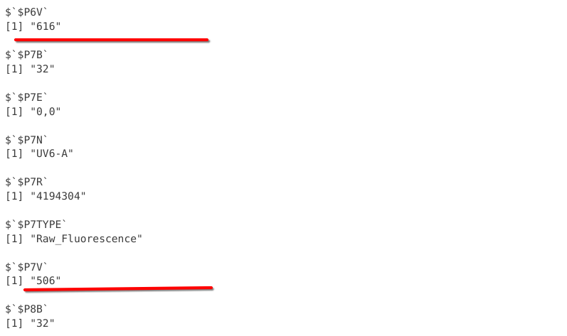
Fortunately for all involved, there is a consistently repeating pattern for the keywords corresponding to each detector. We can see that here for $P7B, $P7E, $P7N, $P7R, $P7TYPE, $P7V
.
When referencing to the Flow Cytometry Standard documentation, here are what the particular keyword letters mean:
B
Number of bits reserved for parameter number n
E
Amplification type for parameter n.
N
Short Name for parameter n.
R
Range for parameter number n.
TYPE
Detector type for parameter n.
V
Detector voltage for parameter n.
.
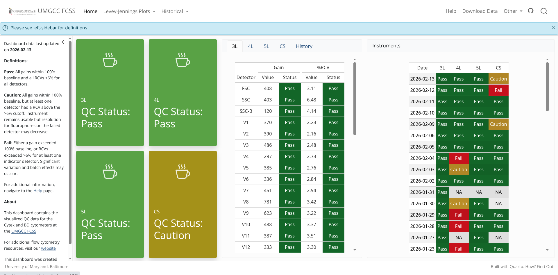
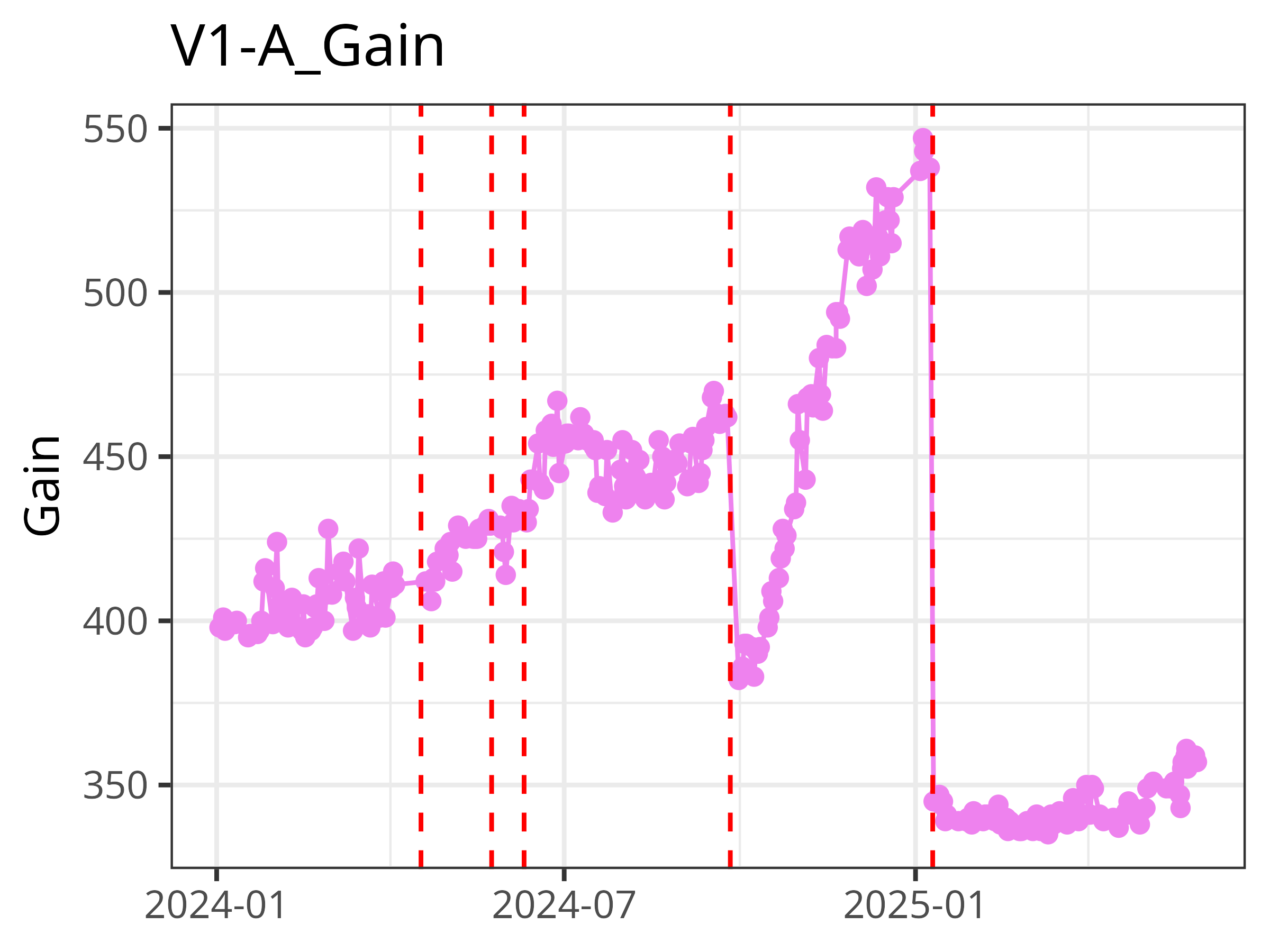
While not immediately obvious, understanding what these keywords encoded has proven useful for our core. In our case, we have built an automated InstrumentQC dashboard for all the instruments at our core.
.
By extracting out from our daily QC bead .fcs files the stored N (Detector Name) and V (Gain/Voltage) values for all the individual detectors, it allows us to plot Levey-Jennings Plots for our individual instruments, giving us usually around a months warning before an individual laser begins to fail. This helps with scheduling the Field-Service Engineer visit before it starts impacting the actual data.
.
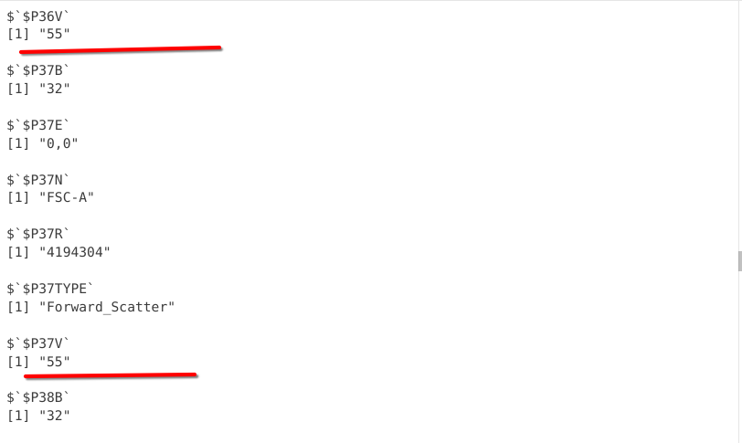
While most of the detectors keywords are similar (only changing there individual name and voltage) there are a couple exceptions.
.
For the FSC/SSC parameters, instead of Raw_Fluorescence value for Type, we see the corresponding Scatter value get return. This in term is what is used by various commercial softwares to show those axis as linear instead of biexponential when selected.
.
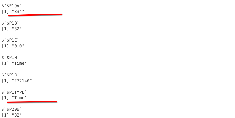
This is similarly the case for the Time parameter, where in addition to Type being set to Time, the range also appears different to Raw/Scatters value.
Middle Metadata
.
Once we are out of the detector keywords, we find the last of the $Metadata associated keywords.
$`$PAR`
[1] "61"
$`$PROJ`
[1] "CellCounts4L_AB_05"
$`$SPILLOVER`
UV1-A UV2-A UV3-A UV4-A UV5-A UV6-A UV7-A UV8-A UV9-A UV10-A UV11-A
[1,] 1e+00 0 0 0 0 0 0 0 0 0 0
[2,] 1e-06 1 0 0 0 0 0 0 0 0 0
[3,] 0e+00 0 1 0 0 0 0 0 0 0 0
[4,] 0e+00 0 0 1 0 0 0 0 0 0 0
[5,] 0e+00 0 0 0 1 0 0 0 0 0 0
[6,] 0e+00 0 0 0 0 1 0 0 0 0 0
[7,] 0e+00 0 0 0 0 0 1 0 0 0 0
[8,] 0e+00 0 0 0 0 0 0 1 0 0 0
[9,] 0e+00 0 0 0 0 0 0 0 1 0 0
[10,] 0e+00 0 0 0 0 0 0 0 0 1 0
[11,] 0e+00 0 0 0 0 0 0 0 0 0 1
[12,] 0e+00 0 0 0 0 0 0 0 0 0 0
[13,] 0e+00 0 0 0 0 0 0 0 0 0 0
[14,] 0e+00 0 0 0 0 0 0 0 0 0 0
[15,] 0e+00 0 0 0 0 0 0 0 0 0 0
[16,] 0e+00 0 0 0 0 0 0 0 0 0 0
[17,] 0e+00 0 0 0 0 0 0 0 0 0 0
[18,] 0e+00 0 0 0 0 0 0 0 0 0 0
[19,] 0e+00 0 0 0 0 0 0 0 0 0 0
[20,] 0e+00 0 0 0 0 0 0 0 0 0 0
[21,] 0e+00 0 0 0 0 0 0 0 0 0 0
[22,] 0e+00 0 0 0 0 0 0 0 0 0 0
[23,] 0e+00 0 0 0 0 0 0 0 0 0 0
[24,] 0e+00 0 0 0 0 0 0 0 0 0 0
[25,] 0e+00 0 0 0 0 0 0 0 0 0 0
[26,] 0e+00 0 0 0 0 0 0 0 0 0 0
[27,] 0e+00 0 0 0 0 0 0 0 0 0 0
[28,] 0e+00 0 0 0 0 0 0 0 0 0 0
[29,] 0e+00 0 0 0 0 0 0 0 0 0 0
[30,] 0e+00 0 0 0 0 0 0 0 0 0 0
[31,] 0e+00 0 0 0 0 0 0 0 0 0 0
[32,] 0e+00 0 0 0 0 0 0 0 0 0 0
[33,] 0e+00 0 0 0 0 0 0 0 0 0 0
[34,] 0e+00 0 0 0 0 0 0 0 0 0 0
[35,] 0e+00 0 0 0 0 0 0 0 0 0 0
[36,] 0e+00 0 0 0 0 0 0 0 0 0 0
[37,] 0e+00 0 0 0 0 0 0 0 0 0 0
[38,] 0e+00 0 0 0 0 0 0 0 0 0 0
[39,] 0e+00 0 0 0 0 0 0 0 0 0 0
[40,] 0e+00 0 0 0 0 0 0 0 0 0 0
[41,] 0e+00 0 0 0 0 0 0 0 0 0 0
[42,] 0e+00 0 0 0 0 0 0 0 0 0 0
[43,] 0e+00 0 0 0 0 0 0 0 0 0 0
[44,] 0e+00 0 0 0 0 0 0 0 0 0 0
[45,] 0e+00 0 0 0 0 0 0 0 0 0 0
[46,] 0e+00 0 0 0 0 0 0 0 0 0 0
[47,] 0e+00 0 0 0 0 0 0 0 0 0 0
[48,] 0e+00 0 0 0 0 0 0 0 0 0 0
[49,] 0e+00 0 0 0 0 0 0 0 0 0 0
[50,] 0e+00 0 0 0 0 0 0 0 0 0 0
[51,] 0e+00 0 0 0 0 0 0 0 0 0 0
[52,] 0e+00 0 0 0 0 0 0 0 0 0 0
[53,] 0e+00 0 0 0 0 0 0 0 0 0 0
[54,] 0e+00 0 0 0 0 0 0 0 0 0 0
UV12-A UV13-A UV14-A UV15-A UV16-A V1-A V2-A V3-A V4-A V5-A V6-A V7-A
[1,] 0 0 0 0 0 0 0 0 0 0 0 0
[2,] 0 0 0 0 0 0 0 0 0 0 0 0
[3,] 0 0 0 0 0 0 0 0 0 0 0 0
[4,] 0 0 0 0 0 0 0 0 0 0 0 0
[5,] 0 0 0 0 0 0 0 0 0 0 0 0
[6,] 0 0 0 0 0 0 0 0 0 0 0 0
[7,] 0 0 0 0 0 0 0 0 0 0 0 0
[8,] 0 0 0 0 0 0 0 0 0 0 0 0
[9,] 0 0 0 0 0 0 0 0 0 0 0 0
[10,] 0 0 0 0 0 0 0 0 0 0 0 0
[11,] 0 0 0 0 0 0 0 0 0 0 0 0
[12,] 1 0 0 0 0 0 0 0 0 0 0 0
[13,] 0 1 0 0 0 0 0 0 0 0 0 0
[14,] 0 0 1 0 0 0 0 0 0 0 0 0
[15,] 0 0 0 1 0 0 0 0 0 0 0 0
[16,] 0 0 0 0 1 0 0 0 0 0 0 0
[17,] 0 0 0 0 0 1 0 0 0 0 0 0
[18,] 0 0 0 0 0 0 1 0 0 0 0 0
[19,] 0 0 0 0 0 0 0 1 0 0 0 0
[20,] 0 0 0 0 0 0 0 0 1 0 0 0
[21,] 0 0 0 0 0 0 0 0 0 1 0 0
[22,] 0 0 0 0 0 0 0 0 0 0 1 0
[23,] 0 0 0 0 0 0 0 0 0 0 0 1
[24,] 0 0 0 0 0 0 0 0 0 0 0 0
[25,] 0 0 0 0 0 0 0 0 0 0 0 0
[26,] 0 0 0 0 0 0 0 0 0 0 0 0
[27,] 0 0 0 0 0 0 0 0 0 0 0 0
[28,] 0 0 0 0 0 0 0 0 0 0 0 0
[29,] 0 0 0 0 0 0 0 0 0 0 0 0
[30,] 0 0 0 0 0 0 0 0 0 0 0 0
[31,] 0 0 0 0 0 0 0 0 0 0 0 0
[32,] 0 0 0 0 0 0 0 0 0 0 0 0
[33,] 0 0 0 0 0 0 0 0 0 0 0 0
[34,] 0 0 0 0 0 0 0 0 0 0 0 0
[35,] 0 0 0 0 0 0 0 0 0 0 0 0
[36,] 0 0 0 0 0 0 0 0 0 0 0 0
[37,] 0 0 0 0 0 0 0 0 0 0 0 0
[38,] 0 0 0 0 0 0 0 0 0 0 0 0
[39,] 0 0 0 0 0 0 0 0 0 0 0 0
[40,] 0 0 0 0 0 0 0 0 0 0 0 0
[41,] 0 0 0 0 0 0 0 0 0 0 0 0
[42,] 0 0 0 0 0 0 0 0 0 0 0 0
[43,] 0 0 0 0 0 0 0 0 0 0 0 0
[44,] 0 0 0 0 0 0 0 0 0 0 0 0
[45,] 0 0 0 0 0 0 0 0 0 0 0 0
[46,] 0 0 0 0 0 0 0 0 0 0 0 0
[47,] 0 0 0 0 0 0 0 0 0 0 0 0
[48,] 0 0 0 0 0 0 0 0 0 0 0 0
[49,] 0 0 0 0 0 0 0 0 0 0 0 0
[50,] 0 0 0 0 0 0 0 0 0 0 0 0
[51,] 0 0 0 0 0 0 0 0 0 0 0 0
[52,] 0 0 0 0 0 0 0 0 0 0 0 0
[53,] 0 0 0 0 0 0 0 0 0 0 0 0
[54,] 0 0 0 0 0 0 0 0 0 0 0 0
V8-A V9-A V10-A V11-A V12-A V13-A V14-A V15-A V16-A B1-A B2-A B3-A B4-A
[1,] 0 0 0 0 0 0 0 0 0 0 0 0 0
[2,] 0 0 0 0 0 0 0 0 0 0 0 0 0
[3,] 0 0 0 0 0 0 0 0 0 0 0 0 0
[4,] 0 0 0 0 0 0 0 0 0 0 0 0 0
[5,] 0 0 0 0 0 0 0 0 0 0 0 0 0
[6,] 0 0 0 0 0 0 0 0 0 0 0 0 0
[7,] 0 0 0 0 0 0 0 0 0 0 0 0 0
[8,] 0 0 0 0 0 0 0 0 0 0 0 0 0
[9,] 0 0 0 0 0 0 0 0 0 0 0 0 0
[10,] 0 0 0 0 0 0 0 0 0 0 0 0 0
[11,] 0 0 0 0 0 0 0 0 0 0 0 0 0
[12,] 0 0 0 0 0 0 0 0 0 0 0 0 0
[13,] 0 0 0 0 0 0 0 0 0 0 0 0 0
[14,] 0 0 0 0 0 0 0 0 0 0 0 0 0
[15,] 0 0 0 0 0 0 0 0 0 0 0 0 0
[16,] 0 0 0 0 0 0 0 0 0 0 0 0 0
[17,] 0 0 0 0 0 0 0 0 0 0 0 0 0
[18,] 0 0 0 0 0 0 0 0 0 0 0 0 0
[19,] 0 0 0 0 0 0 0 0 0 0 0 0 0
[20,] 0 0 0 0 0 0 0 0 0 0 0 0 0
[21,] 0 0 0 0 0 0 0 0 0 0 0 0 0
[22,] 0 0 0 0 0 0 0 0 0 0 0 0 0
[23,] 0 0 0 0 0 0 0 0 0 0 0 0 0
[24,] 1 0 0 0 0 0 0 0 0 0 0 0 0
[25,] 0 1 0 0 0 0 0 0 0 0 0 0 0
[26,] 0 0 1 0 0 0 0 0 0 0 0 0 0
[27,] 0 0 0 1 0 0 0 0 0 0 0 0 0
[28,] 0 0 0 0 1 0 0 0 0 0 0 0 0
[29,] 0 0 0 0 0 1 0 0 0 0 0 0 0
[30,] 0 0 0 0 0 0 1 0 0 0 0 0 0
[31,] 0 0 0 0 0 0 0 1 0 0 0 0 0
[32,] 0 0 0 0 0 0 0 0 1 0 0 0 0
[33,] 0 0 0 0 0 0 0 0 0 1 0 0 0
[34,] 0 0 0 0 0 0 0 0 0 0 1 0 0
[35,] 0 0 0 0 0 0 0 0 0 0 0 1 0
[36,] 0 0 0 0 0 0 0 0 0 0 0 0 1
[37,] 0 0 0 0 0 0 0 0 0 0 0 0 0
[38,] 0 0 0 0 0 0 0 0 0 0 0 0 0
[39,] 0 0 0 0 0 0 0 0 0 0 0 0 0
[40,] 0 0 0 0 0 0 0 0 0 0 0 0 0
[41,] 0 0 0 0 0 0 0 0 0 0 0 0 0
[42,] 0 0 0 0 0 0 0 0 0 0 0 0 0
[43,] 0 0 0 0 0 0 0 0 0 0 0 0 0
[44,] 0 0 0 0 0 0 0 0 0 0 0 0 0
[45,] 0 0 0 0 0 0 0 0 0 0 0 0 0
[46,] 0 0 0 0 0 0 0 0 0 0 0 0 0
[47,] 0 0 0 0 0 0 0 0 0 0 0 0 0
[48,] 0 0 0 0 0 0 0 0 0 0 0 0 0
[49,] 0 0 0 0 0 0 0 0 0 0 0 0 0
[50,] 0 0 0 0 0 0 0 0 0 0 0 0 0
[51,] 0 0 0 0 0 0 0 0 0 0 0 0 0
[52,] 0 0 0 0 0 0 0 0 0 0 0 0 0
[53,] 0 0 0 0 0 0 0 0 0 0 0 0 0
[54,] 0 0 0 0 0 0 0 0 0 0 0 0 0
B5-A B6-A B7-A B8-A B9-A B10-A B11-A B12-A B13-A B14-A R1-A R2-A R3-A
[1,] 0 0 0 0 0 0 0 0 0 0 0 0 0
[2,] 0 0 0 0 0 0 0 0 0 0 0 0 0
[3,] 0 0 0 0 0 0 0 0 0 0 0 0 0
[4,] 0 0 0 0 0 0 0 0 0 0 0 0 0
[5,] 0 0 0 0 0 0 0 0 0 0 0 0 0
[6,] 0 0 0 0 0 0 0 0 0 0 0 0 0
[7,] 0 0 0 0 0 0 0 0 0 0 0 0 0
[8,] 0 0 0 0 0 0 0 0 0 0 0 0 0
[9,] 0 0 0 0 0 0 0 0 0 0 0 0 0
[10,] 0 0 0 0 0 0 0 0 0 0 0 0 0
[11,] 0 0 0 0 0 0 0 0 0 0 0 0 0
[12,] 0 0 0 0 0 0 0 0 0 0 0 0 0
[13,] 0 0 0 0 0 0 0 0 0 0 0 0 0
[14,] 0 0 0 0 0 0 0 0 0 0 0 0 0
[15,] 0 0 0 0 0 0 0 0 0 0 0 0 0
[16,] 0 0 0 0 0 0 0 0 0 0 0 0 0
[17,] 0 0 0 0 0 0 0 0 0 0 0 0 0
[18,] 0 0 0 0 0 0 0 0 0 0 0 0 0
[19,] 0 0 0 0 0 0 0 0 0 0 0 0 0
[20,] 0 0 0 0 0 0 0 0 0 0 0 0 0
[21,] 0 0 0 0 0 0 0 0 0 0 0 0 0
[22,] 0 0 0 0 0 0 0 0 0 0 0 0 0
[23,] 0 0 0 0 0 0 0 0 0 0 0 0 0
[24,] 0 0 0 0 0 0 0 0 0 0 0 0 0
[25,] 0 0 0 0 0 0 0 0 0 0 0 0 0
[26,] 0 0 0 0 0 0 0 0 0 0 0 0 0
[27,] 0 0 0 0 0 0 0 0 0 0 0 0 0
[28,] 0 0 0 0 0 0 0 0 0 0 0 0 0
[29,] 0 0 0 0 0 0 0 0 0 0 0 0 0
[30,] 0 0 0 0 0 0 0 0 0 0 0 0 0
[31,] 0 0 0 0 0 0 0 0 0 0 0 0 0
[32,] 0 0 0 0 0 0 0 0 0 0 0 0 0
[33,] 0 0 0 0 0 0 0 0 0 0 0 0 0
[34,] 0 0 0 0 0 0 0 0 0 0 0 0 0
[35,] 0 0 0 0 0 0 0 0 0 0 0 0 0
[36,] 0 0 0 0 0 0 0 0 0 0 0 0 0
[37,] 1 0 0 0 0 0 0 0 0 0 0 0 0
[38,] 0 1 0 0 0 0 0 0 0 0 0 0 0
[39,] 0 0 1 0 0 0 0 0 0 0 0 0 0
[40,] 0 0 0 1 0 0 0 0 0 0 0 0 0
[41,] 0 0 0 0 1 0 0 0 0 0 0 0 0
[42,] 0 0 0 0 0 1 0 0 0 0 0 0 0
[43,] 0 0 0 0 0 0 1 0 0 0 0 0 0
[44,] 0 0 0 0 0 0 0 1 0 0 0 0 0
[45,] 0 0 0 0 0 0 0 0 1 0 0 0 0
[46,] 0 0 0 0 0 0 0 0 0 1 0 0 0
[47,] 0 0 0 0 0 0 0 0 0 0 1 0 0
[48,] 0 0 0 0 0 0 0 0 0 0 0 1 0
[49,] 0 0 0 0 0 0 0 0 0 0 0 0 1
[50,] 0 0 0 0 0 0 0 0 0 0 0 0 0
[51,] 0 0 0 0 0 0 0 0 0 0 0 0 0
[52,] 0 0 0 0 0 0 0 0 0 0 0 0 0
[53,] 0 0 0 0 0 0 0 0 0 0 0 0 0
[54,] 0 0 0 0 0 0 0 0 0 0 0 0 0
R4-A R5-A R6-A R7-A R8-A
[1,] 0 0 0 0 0
[2,] 0 0 0 0 0
[3,] 0 0 0 0 0
[4,] 0 0 0 0 0
[5,] 0 0 0 0 0
[6,] 0 0 0 0 0
[7,] 0 0 0 0 0
[8,] 0 0 0 0 0
[9,] 0 0 0 0 0
[10,] 0 0 0 0 0
[11,] 0 0 0 0 0
[12,] 0 0 0 0 0
[13,] 0 0 0 0 0
[14,] 0 0 0 0 0
[15,] 0 0 0 0 0
[16,] 0 0 0 0 0
[17,] 0 0 0 0 0
[18,] 0 0 0 0 0
[19,] 0 0 0 0 0
[20,] 0 0 0 0 0
[21,] 0 0 0 0 0
[22,] 0 0 0 0 0
[23,] 0 0 0 0 0
[24,] 0 0 0 0 0
[25,] 0 0 0 0 0
[26,] 0 0 0 0 0
[27,] 0 0 0 0 0
[28,] 0 0 0 0 0
[29,] 0 0 0 0 0
[30,] 0 0 0 0 0
[31,] 0 0 0 0 0
[32,] 0 0 0 0 0
[33,] 0 0 0 0 0
[34,] 0 0 0 0 0
[35,] 0 0 0 0 0
[36,] 0 0 0 0 0
[37,] 0 0 0 0 0
[38,] 0 0 0 0 0
[39,] 0 0 0 0 0
[40,] 0 0 0 0 0
[41,] 0 0 0 0 0
[42,] 0 0 0 0 0
[43,] 0 0 0 0 0
[44,] 0 0 0 0 0
[45,] 0 0 0 0 0
[46,] 0 0 0 0 0
[47,] 0 0 0 0 0
[48,] 0 0 0 0 0
[49,] 0 0 0 0 0
[50,] 1 0 0 0 0
[51,] 0 1 0 0 0
[52,] 0 0 1 0 0
[53,] 0 0 0 1 0
[54,] 0 0 0 0 1
$`$TIMESTEP`
[1] "0.0001"
$`$TOT`
[1] "100"
$`$VOL`
[1] "30.31"
$`APPLY COMPENSATION`
[1] "FALSE"
$CHARSET
[1] "utf-8"
$CREATOR
[1] "SpectroFlo 3.3.0"
$FCSversion
[1] "3"
$FILENAME
[1] "data/CellCounts4L_AB_05_ND050_05.fcs"
$`FSC ASF`
[1] "1.21"
$GROUPNAME
[1] "ND050"
$GUID
[1] "CellCounts4L_AB_05-ND050-05.fcs".
Among those of potential interest
Proj
Often corresponding to the experiment file name
Spillover
Where the internal spillover matrix is stored (we will revisit during compensation)
UV1-A UV2-A UV3-A UV4-A UV5-A UV6-A UV7-A UV8-A UV9-A UV10-A UV11-A
[1,] 1e+00 0 0 0 0 0 0 0 0 0 0
[2,] 1e-06 1 0 0 0 0 0 0 0 0 0
[3,] 0e+00 0 1 0 0 0 0 0 0 0 0
[4,] 0e+00 0 0 1 0 0 0 0 0 0 0
[5,] 0e+00 0 0 0 1 0 0 0 0 0 0
[6,] 0e+00 0 0 0 0 1 0 0 0 0 0
[7,] 0e+00 0 0 0 0 0 1 0 0 0 0
[8,] 0e+00 0 0 0 0 0 0 1 0 0 0
[9,] 0e+00 0 0 0 0 0 0 0 1 0 0
[10,] 0e+00 0 0 0 0 0 0 0 0 1 0
[11,] 0e+00 0 0 0 0 0 0 0 0 0 1
[12,] 0e+00 0 0 0 0 0 0 0 0 0 0
[13,] 0e+00 0 0 0 0 0 0 0 0 0 0
[14,] 0e+00 0 0 0 0 0 0 0 0 0 0
[15,] 0e+00 0 0 0 0 0 0 0 0 0 0
[16,] 0e+00 0 0 0 0 0 0 0 0 0 0
[17,] 0e+00 0 0 0 0 0 0 0 0 0 0
[18,] 0e+00 0 0 0 0 0 0 0 0 0 0
[19,] 0e+00 0 0 0 0 0 0 0 0 0 0
[20,] 0e+00 0 0 0 0 0 0 0 0 0 0
[21,] 0e+00 0 0 0 0 0 0 0 0 0 0
[22,] 0e+00 0 0 0 0 0 0 0 0 0 0
[23,] 0e+00 0 0 0 0 0 0 0 0 0 0
[24,] 0e+00 0 0 0 0 0 0 0 0 0 0
[25,] 0e+00 0 0 0 0 0 0 0 0 0 0
[26,] 0e+00 0 0 0 0 0 0 0 0 0 0
[27,] 0e+00 0 0 0 0 0 0 0 0 0 0
[28,] 0e+00 0 0 0 0 0 0 0 0 0 0
[29,] 0e+00 0 0 0 0 0 0 0 0 0 0
[30,] 0e+00 0 0 0 0 0 0 0 0 0 0
[31,] 0e+00 0 0 0 0 0 0 0 0 0 0
[32,] 0e+00 0 0 0 0 0 0 0 0 0 0
[33,] 0e+00 0 0 0 0 0 0 0 0 0 0
[34,] 0e+00 0 0 0 0 0 0 0 0 0 0
[35,] 0e+00 0 0 0 0 0 0 0 0 0 0
[36,] 0e+00 0 0 0 0 0 0 0 0 0 0
[37,] 0e+00 0 0 0 0 0 0 0 0 0 0
[38,] 0e+00 0 0 0 0 0 0 0 0 0 0
[39,] 0e+00 0 0 0 0 0 0 0 0 0 0
[40,] 0e+00 0 0 0 0 0 0 0 0 0 0
[41,] 0e+00 0 0 0 0 0 0 0 0 0 0
[42,] 0e+00 0 0 0 0 0 0 0 0 0 0
[43,] 0e+00 0 0 0 0 0 0 0 0 0 0
[44,] 0e+00 0 0 0 0 0 0 0 0 0 0
[45,] 0e+00 0 0 0 0 0 0 0 0 0 0
[46,] 0e+00 0 0 0 0 0 0 0 0 0 0
[47,] 0e+00 0 0 0 0 0 0 0 0 0 0
[48,] 0e+00 0 0 0 0 0 0 0 0 0 0
[49,] 0e+00 0 0 0 0 0 0 0 0 0 0
[50,] 0e+00 0 0 0 0 0 0 0 0 0 0
[51,] 0e+00 0 0 0 0 0 0 0 0 0 0
[52,] 0e+00 0 0 0 0 0 0 0 0 0 0
[53,] 0e+00 0 0 0 0 0 0 0 0 0 0
[54,] 0e+00 0 0 0 0 0 0 0 0 0 0
UV12-A UV13-A UV14-A UV15-A UV16-A V1-A V2-A V3-A V4-A V5-A V6-A V7-A
[1,] 0 0 0 0 0 0 0 0 0 0 0 0
[2,] 0 0 0 0 0 0 0 0 0 0 0 0
[3,] 0 0 0 0 0 0 0 0 0 0 0 0
[4,] 0 0 0 0 0 0 0 0 0 0 0 0
[5,] 0 0 0 0 0 0 0 0 0 0 0 0
[6,] 0 0 0 0 0 0 0 0 0 0 0 0
[7,] 0 0 0 0 0 0 0 0 0 0 0 0
[8,] 0 0 0 0 0 0 0 0 0 0 0 0
[9,] 0 0 0 0 0 0 0 0 0 0 0 0
[10,] 0 0 0 0 0 0 0 0 0 0 0 0
[11,] 0 0 0 0 0 0 0 0 0 0 0 0
[12,] 1 0 0 0 0 0 0 0 0 0 0 0
[13,] 0 1 0 0 0 0 0 0 0 0 0 0
[14,] 0 0 1 0 0 0 0 0 0 0 0 0
[15,] 0 0 0 1 0 0 0 0 0 0 0 0
[16,] 0 0 0 0 1 0 0 0 0 0 0 0
[17,] 0 0 0 0 0 1 0 0 0 0 0 0
[18,] 0 0 0 0 0 0 1 0 0 0 0 0
[19,] 0 0 0 0 0 0 0 1 0 0 0 0
[20,] 0 0 0 0 0 0 0 0 1 0 0 0
[21,] 0 0 0 0 0 0 0 0 0 1 0 0
[22,] 0 0 0 0 0 0 0 0 0 0 1 0
[23,] 0 0 0 0 0 0 0 0 0 0 0 1
[24,] 0 0 0 0 0 0 0 0 0 0 0 0
[25,] 0 0 0 0 0 0 0 0 0 0 0 0
[26,] 0 0 0 0 0 0 0 0 0 0 0 0
[27,] 0 0 0 0 0 0 0 0 0 0 0 0
[28,] 0 0 0 0 0 0 0 0 0 0 0 0
[29,] 0 0 0 0 0 0 0 0 0 0 0 0
[30,] 0 0 0 0 0 0 0 0 0 0 0 0
[31,] 0 0 0 0 0 0 0 0 0 0 0 0
[32,] 0 0 0 0 0 0 0 0 0 0 0 0
[33,] 0 0 0 0 0 0 0 0 0 0 0 0
[34,] 0 0 0 0 0 0 0 0 0 0 0 0
[35,] 0 0 0 0 0 0 0 0 0 0 0 0
[36,] 0 0 0 0 0 0 0 0 0 0 0 0
[37,] 0 0 0 0 0 0 0 0 0 0 0 0
[38,] 0 0 0 0 0 0 0 0 0 0 0 0
[39,] 0 0 0 0 0 0 0 0 0 0 0 0
[40,] 0 0 0 0 0 0 0 0 0 0 0 0
[41,] 0 0 0 0 0 0 0 0 0 0 0 0
[42,] 0 0 0 0 0 0 0 0 0 0 0 0
[43,] 0 0 0 0 0 0 0 0 0 0 0 0
[44,] 0 0 0 0 0 0 0 0 0 0 0 0
[45,] 0 0 0 0 0 0 0 0 0 0 0 0
[46,] 0 0 0 0 0 0 0 0 0 0 0 0
[47,] 0 0 0 0 0 0 0 0 0 0 0 0
[48,] 0 0 0 0 0 0 0 0 0 0 0 0
[49,] 0 0 0 0 0 0 0 0 0 0 0 0
[50,] 0 0 0 0 0 0 0 0 0 0 0 0
[51,] 0 0 0 0 0 0 0 0 0 0 0 0
[52,] 0 0 0 0 0 0 0 0 0 0 0 0
[53,] 0 0 0 0 0 0 0 0 0 0 0 0
[54,] 0 0 0 0 0 0 0 0 0 0 0 0
V8-A V9-A V10-A V11-A V12-A V13-A V14-A V15-A V16-A B1-A B2-A B3-A B4-A
[1,] 0 0 0 0 0 0 0 0 0 0 0 0 0
[2,] 0 0 0 0 0 0 0 0 0 0 0 0 0
[3,] 0 0 0 0 0 0 0 0 0 0 0 0 0
[4,] 0 0 0 0 0 0 0 0 0 0 0 0 0
[5,] 0 0 0 0 0 0 0 0 0 0 0 0 0
[6,] 0 0 0 0 0 0 0 0 0 0 0 0 0
[7,] 0 0 0 0 0 0 0 0 0 0 0 0 0
[8,] 0 0 0 0 0 0 0 0 0 0 0 0 0
[9,] 0 0 0 0 0 0 0 0 0 0 0 0 0
[10,] 0 0 0 0 0 0 0 0 0 0 0 0 0
[11,] 0 0 0 0 0 0 0 0 0 0 0 0 0
[12,] 0 0 0 0 0 0 0 0 0 0 0 0 0
[13,] 0 0 0 0 0 0 0 0 0 0 0 0 0
[14,] 0 0 0 0 0 0 0 0 0 0 0 0 0
[15,] 0 0 0 0 0 0 0 0 0 0 0 0 0
[16,] 0 0 0 0 0 0 0 0 0 0 0 0 0
[17,] 0 0 0 0 0 0 0 0 0 0 0 0 0
[18,] 0 0 0 0 0 0 0 0 0 0 0 0 0
[19,] 0 0 0 0 0 0 0 0 0 0 0 0 0
[20,] 0 0 0 0 0 0 0 0 0 0 0 0 0
[21,] 0 0 0 0 0 0 0 0 0 0 0 0 0
[22,] 0 0 0 0 0 0 0 0 0 0 0 0 0
[23,] 0 0 0 0 0 0 0 0 0 0 0 0 0
[24,] 1 0 0 0 0 0 0 0 0 0 0 0 0
[25,] 0 1 0 0 0 0 0 0 0 0 0 0 0
[26,] 0 0 1 0 0 0 0 0 0 0 0 0 0
[27,] 0 0 0 1 0 0 0 0 0 0 0 0 0
[28,] 0 0 0 0 1 0 0 0 0 0 0 0 0
[29,] 0 0 0 0 0 1 0 0 0 0 0 0 0
[30,] 0 0 0 0 0 0 1 0 0 0 0 0 0
[31,] 0 0 0 0 0 0 0 1 0 0 0 0 0
[32,] 0 0 0 0 0 0 0 0 1 0 0 0 0
[33,] 0 0 0 0 0 0 0 0 0 1 0 0 0
[34,] 0 0 0 0 0 0 0 0 0 0 1 0 0
[35,] 0 0 0 0 0 0 0 0 0 0 0 1 0
[36,] 0 0 0 0 0 0 0 0 0 0 0 0 1
[37,] 0 0 0 0 0 0 0 0 0 0 0 0 0
[38,] 0 0 0 0 0 0 0 0 0 0 0 0 0
[39,] 0 0 0 0 0 0 0 0 0 0 0 0 0
[40,] 0 0 0 0 0 0 0 0 0 0 0 0 0
[41,] 0 0 0 0 0 0 0 0 0 0 0 0 0
[42,] 0 0 0 0 0 0 0 0 0 0 0 0 0
[43,] 0 0 0 0 0 0 0 0 0 0 0 0 0
[44,] 0 0 0 0 0 0 0 0 0 0 0 0 0
[45,] 0 0 0 0 0 0 0 0 0 0 0 0 0
[46,] 0 0 0 0 0 0 0 0 0 0 0 0 0
[47,] 0 0 0 0 0 0 0 0 0 0 0 0 0
[48,] 0 0 0 0 0 0 0 0 0 0 0 0 0
[49,] 0 0 0 0 0 0 0 0 0 0 0 0 0
[50,] 0 0 0 0 0 0 0 0 0 0 0 0 0
[51,] 0 0 0 0 0 0 0 0 0 0 0 0 0
[52,] 0 0 0 0 0 0 0 0 0 0 0 0 0
[53,] 0 0 0 0 0 0 0 0 0 0 0 0 0
[54,] 0 0 0 0 0 0 0 0 0 0 0 0 0
B5-A B6-A B7-A B8-A B9-A B10-A B11-A B12-A B13-A B14-A R1-A R2-A R3-A
[1,] 0 0 0 0 0 0 0 0 0 0 0 0 0
[2,] 0 0 0 0 0 0 0 0 0 0 0 0 0
[3,] 0 0 0 0 0 0 0 0 0 0 0 0 0
[4,] 0 0 0 0 0 0 0 0 0 0 0 0 0
[5,] 0 0 0 0 0 0 0 0 0 0 0 0 0
[6,] 0 0 0 0 0 0 0 0 0 0 0 0 0
[7,] 0 0 0 0 0 0 0 0 0 0 0 0 0
[8,] 0 0 0 0 0 0 0 0 0 0 0 0 0
[9,] 0 0 0 0 0 0 0 0 0 0 0 0 0
[10,] 0 0 0 0 0 0 0 0 0 0 0 0 0
[11,] 0 0 0 0 0 0 0 0 0 0 0 0 0
[12,] 0 0 0 0 0 0 0 0 0 0 0 0 0
[13,] 0 0 0 0 0 0 0 0 0 0 0 0 0
[14,] 0 0 0 0 0 0 0 0 0 0 0 0 0
[15,] 0 0 0 0 0 0 0 0 0 0 0 0 0
[16,] 0 0 0 0 0 0 0 0 0 0 0 0 0
[17,] 0 0 0 0 0 0 0 0 0 0 0 0 0
[18,] 0 0 0 0 0 0 0 0 0 0 0 0 0
[19,] 0 0 0 0 0 0 0 0 0 0 0 0 0
[20,] 0 0 0 0 0 0 0 0 0 0 0 0 0
[21,] 0 0 0 0 0 0 0 0 0 0 0 0 0
[22,] 0 0 0 0 0 0 0 0 0 0 0 0 0
[23,] 0 0 0 0 0 0 0 0 0 0 0 0 0
[24,] 0 0 0 0 0 0 0 0 0 0 0 0 0
[25,] 0 0 0 0 0 0 0 0 0 0 0 0 0
[26,] 0 0 0 0 0 0 0 0 0 0 0 0 0
[27,] 0 0 0 0 0 0 0 0 0 0 0 0 0
[28,] 0 0 0 0 0 0 0 0 0 0 0 0 0
[29,] 0 0 0 0 0 0 0 0 0 0 0 0 0
[30,] 0 0 0 0 0 0 0 0 0 0 0 0 0
[31,] 0 0 0 0 0 0 0 0 0 0 0 0 0
[32,] 0 0 0 0 0 0 0 0 0 0 0 0 0
[33,] 0 0 0 0 0 0 0 0 0 0 0 0 0
[34,] 0 0 0 0 0 0 0 0 0 0 0 0 0
[35,] 0 0 0 0 0 0 0 0 0 0 0 0 0
[36,] 0 0 0 0 0 0 0 0 0 0 0 0 0
[37,] 1 0 0 0 0 0 0 0 0 0 0 0 0
[38,] 0 1 0 0 0 0 0 0 0 0 0 0 0
[39,] 0 0 1 0 0 0 0 0 0 0 0 0 0
[40,] 0 0 0 1 0 0 0 0 0 0 0 0 0
[41,] 0 0 0 0 1 0 0 0 0 0 0 0 0
[42,] 0 0 0 0 0 1 0 0 0 0 0 0 0
[43,] 0 0 0 0 0 0 1 0 0 0 0 0 0
[44,] 0 0 0 0 0 0 0 1 0 0 0 0 0
[45,] 0 0 0 0 0 0 0 0 1 0 0 0 0
[46,] 0 0 0 0 0 0 0 0 0 1 0 0 0
[47,] 0 0 0 0 0 0 0 0 0 0 1 0 0
[48,] 0 0 0 0 0 0 0 0 0 0 0 1 0
[49,] 0 0 0 0 0 0 0 0 0 0 0 0 1
[50,] 0 0 0 0 0 0 0 0 0 0 0 0 0
[51,] 0 0 0 0 0 0 0 0 0 0 0 0 0
[52,] 0 0 0 0 0 0 0 0 0 0 0 0 0
[53,] 0 0 0 0 0 0 0 0 0 0 0 0 0
[54,] 0 0 0 0 0 0 0 0 0 0 0 0 0
R4-A R5-A R6-A R7-A R8-A
[1,] 0 0 0 0 0
[2,] 0 0 0 0 0
[3,] 0 0 0 0 0
[4,] 0 0 0 0 0
[5,] 0 0 0 0 0
[6,] 0 0 0 0 0
[7,] 0 0 0 0 0
[8,] 0 0 0 0 0
[9,] 0 0 0 0 0
[10,] 0 0 0 0 0
[11,] 0 0 0 0 0
[12,] 0 0 0 0 0
[13,] 0 0 0 0 0
[14,] 0 0 0 0 0
[15,] 0 0 0 0 0
[16,] 0 0 0 0 0
[17,] 0 0 0 0 0
[18,] 0 0 0 0 0
[19,] 0 0 0 0 0
[20,] 0 0 0 0 0
[21,] 0 0 0 0 0
[22,] 0 0 0 0 0
[23,] 0 0 0 0 0
[24,] 0 0 0 0 0
[25,] 0 0 0 0 0
[26,] 0 0 0 0 0
[27,] 0 0 0 0 0
[28,] 0 0 0 0 0
[29,] 0 0 0 0 0
[30,] 0 0 0 0 0
[31,] 0 0 0 0 0
[32,] 0 0 0 0 0
[33,] 0 0 0 0 0
[34,] 0 0 0 0 0
[35,] 0 0 0 0 0
[36,] 0 0 0 0 0
[37,] 0 0 0 0 0
[38,] 0 0 0 0 0
[39,] 0 0 0 0 0
[40,] 0 0 0 0 0
[41,] 0 0 0 0 0
[42,] 0 0 0 0 0
[43,] 0 0 0 0 0
[44,] 0 0 0 0 0
[45,] 0 0 0 0 0
[46,] 0 0 0 0 0
[47,] 0 0 0 0 0
[48,] 0 0 0 0 0
[49,] 0 0 0 0 0
[50,] 1 0 0 0 0
[51,] 0 1 0 0 0
[52,] 0 0 1 0 0
[53,] 0 0 0 1 0
[54,] 0 0 0 0 1TOT
Total events (in this case my downsampled 100 cells)
Volume
Volume amount acquired during acquisition.
Software
Software used and version
.
You will notice at this point, the keyword names including a “$” symbol have stopped, so tick marks are no longer required (except when there is a space in the name). The only $ remaining is being used as a selector for a particular item in the list.
FILENAME
Basically the full file.path to the .fcs file of interest.
GROUPNAME
The Name assigned to the acquisition Group.
Laser Metadata
.
Next up, there is a small stretch of keywords containing the values associated with the individual lasers as far as delays and area scaling factors for a particular day (also useful when plotted).
Display
.
Then there is a stretch matching whether a particular detector needs to be displayed as linear (in the case of time and scatter) or as log (for individual detectors).
$P10DISPLAY
[1] "LOG"

$P11DISPLAY
[1] "LOG"

$P12DISPLAY
[1] "LOG"

$P13DISPLAY
[1] "LOG"

$P14DISPLAY
[1] "LOG"

$P15DISPLAY
[1] "LOG"

$P16DISPLAY
[1] "LOG"

$P17DISPLAY
[1] "LOG"

$P18DISPLAY
[1] "LIN"

$P19DISPLAY
[1] "LIN"

$P1DISPLAY
[1] "LOG"

$P20DISPLAY
[1] "LOG"

$P21DISPLAY
[1] "LOG"

$P22DISPLAY
[1] "LOG"

$P23DISPLAY
[1] "LOG"

$P24DISPLAY
[1] "LOG"

$P25DISPLAY
[1] "LOG"

$P26DISPLAY
[1] "LOG"

$P27DISPLAY
[1] "LOG"

$P28DISPLAY
[1] "LOG"

$P29DISPLAY
[1] "LOG"

$P2DISPLAY
[1] "LOG"

$P30DISPLAY
[1] "LOG"

$P31DISPLAY
[1] "LOG"

$P32DISPLAY
[1] "LOG"

$P33DISPLAY
[1] "LOG"

$P34DISPLAY
[1] "LOG"

$P35DISPLAY
[1] "LOG"

$P36DISPLAY
[1] "LIN"

$P37DISPLAY
[1] "LIN"

$P38DISPLAY
[1] "LIN"

$P39DISPLAY
[1] "LIN"

$P3DISPLAY
[1] "LOG"

$P40DISPLAY
[1] "LOG"

$P41DISPLAY
[1] "LOG"

$P42DISPLAY
[1] "LOG"

$P43DISPLAY
[1] "LOG"

$P44DISPLAY
[1] "LOG"

$P45DISPLAY
[1] "LOG"

$P46DISPLAY
[1] "LOG"

$P47DISPLAY
[1] "LOG"

$P48DISPLAY
[1] "LOG"

$P49DISPLAY
[1] "LOG"

$P4DISPLAY
[1] "LOG"

$P50DISPLAY
[1] "LOG"

$P51DISPLAY
[1] "LOG"

$P52DISPLAY
[1] "LOG"

$P53DISPLAY
[1] "LOG"

$P54DISPLAY
[1] "LOG"

$P55DISPLAY
[1] "LOG"

$P56DISPLAY
[1] "LOG"

$P57DISPLAY
[1] "LOG"

$P58DISPLAY
[1] "LOG"

$P59DISPLAY
[1] "LOG"

$P5DISPLAY
[1] "LOG"

$P60DISPLAY
[1] "LOG"

$P61DISPLAY
[1] "LOG"

$P6DISPLAY
[1] "LOG"

$P7DISPLAY
[1] "LOG"

$P8DISPLAY
[1] "LOG"

$P9DISPLAY
[1] "LOG"
.
And a few final keywords with threshold, window scaling and other user selected settings.
flowCore Parameters
.
Depending on the arguments selected during read.FCS(), we might also encounter additional keywords that are added in by flowCore. For example, we do not see these keywords when “transformation” is set to FALSE.
flowFrame object 'CellCounts4L_AB_05-ND050-05.fcs'
with 100 cells and 61 observables:
       name   desc     range  minRange  maxRange
$P1    Time     NA    272140         0    272139
$P2   UV1-A     NA   4194304      -111   4194303
$P3   UV2-A     NA   4194304      -111   4194303
$P4   UV3-A     NA   4194304      -111   4194303
$P5   UV4-A     NA   4194304      -111   4194303
...     ...    ...       ...       ...       ...
$P57   R4-A     NA   4194304      -111   4194303
$P58   R5-A     NA   4194304      -111   4194303
$P59   R6-A     NA   4194304      -111   4194303
$P60   R7-A     NA   4194304      -111   4194303
$P61   R8-A     NA   4194304      -111   4194303
476 keywords are stored in the 'description' slot.
By contrast, if we had set “transformation” to TRUE:
flowFrame object 'CellCounts4L_AB_05-ND050-05.fcs'
with 100 cells and 61 observables:
       name   desc     range  minRange  maxRange
$P1    Time     NA    272140         0    272139
$P2   UV1-A     NA   4194304      -111   4194303
$P3   UV2-A     NA   4194304      -111   4194303
$P4   UV3-A     NA   4194304      -111   4194303
$P5   UV4-A     NA   4194304      -111   4194303
...     ...    ...       ...       ...       ...
$P57   R4-A     NA   4194304      -111   4194303
$P58   R5-A     NA   4194304      -111   4194303
$P59   R6-A     NA   4194304      -111   4194303
$P60   R7-A     NA   4194304      -111   4194303
$P61   R8-A     NA   4194304      -111   4194303
599 keywords are stored in the 'description' slot$`WINDOW EXTENSION`
[1] "3"
$transformation
[1] "applied"
$`flowCore_$P1Rmax`
[1] "272140"
$`flowCore_$P1Rmin`
[1] "0"
$`flowCore_$P2Rmax`
[1] "4194304"
$`flowCore_$P2Rmin`
[1] "-111"
$`flowCore_$P3Rmax`
[1] "4194304"
$`flowCore_$P3Rmin`
[1] "-111"
$`flowCore_$P4Rmax`
[1] "4194304"
$`flowCore_$P4Rmin`
[1] "-111"
$`flowCore_$P5Rmax`
[1] "4194304"
$`flowCore_$P5Rmin`
[1] "-111"
$`flowCore_$P6Rmax`
[1] "4194304"
$`flowCore_$P6Rmin`
[1] "-111"
$`flowCore_$P7Rmax`
[1] "4194304"
$`flowCore_$P7Rmin`
[1] "-111"
$`flowCore_$P8Rmax`
[1] "4194304"
$`flowCore_$P8Rmin`
[1] "-26.3464946746826"
$`flowCore_$P9Rmax`
[1] "4194304"
$`flowCore_$P9Rmin`
[1] "-111"
$`flowCore_$P10Rmax`
[1] "4194304"
$`flowCore_$P10Rmin`
[1] "0"
$`flowCore_$P11Rmax`
[1] "4194304"
$`flowCore_$P11Rmin`
[1] "-111"
$`flowCore_$P12Rmax`
[1] "4194304".
For some flow cytometry R packages, you will notice when opening their exported .fcs outputs in commercial software that these flowCore keywords have ended up integrated. It is likely somewhere in the package code the author forgot to add set transformation to FALSE, which is why we are seeing these flowCore keywords after the fact.
Take Away
.
Today we broke open an .fcs file and explored how the underlying data is organized and stored once it is brought into R. In the process, we continued to build familiarity with some of the basic R knowledge, going from smaller simpler objects we encountered in week 2 to matrices and data.frames, to complex objects with multiple slots typical of what we encounter in the Bioconductor packages. We will build on these initial observations on the weeks to come.
.
In context of our continuing analogy, with each function being a tool, and an R package a toolbox, each tool in the toolbox works on different types of objects. A hammer needs nails, screwdrivers need screws, a paintbrush needs paint and a wall, etc. Object types help define these requirements, so when we use a function, knowing what type can help determine what we provide to it in order for it to work properly and not error out.
Additional Resources
Data File Standard for Flow Cytometry, Version FCS 3.1
Take-home Problems
Problem 1
Today’s walkthrough focused on a raw spectral flow cytometry file. Within a subfolder in data you will also find an unmixed .fcs file (2025_07_26…). Using what learned to day, investigate it, and see if you can catalog the main differences that occured to the keyword, parameters and exprs. Did any keywords get added, changed, deleted entirely? etc.
Problem 2
Today’s files were for spectral .fcs files from a Cytek Aurora within a subfolder in data you will also find a conventional flow cytometry file (2025-10_22…). Similarly, explore and see if you find any major differences (beyond the different detector or fluorophore names which will vary based on antibody panel used, etc)
Problem 3
If you have access to commercial software, take one of the .fcs files and try to see if you can see similar internal information from within the software. For those without commercial access, try the equivalent process using Floreada.io.