FCS Clean Up for GitHub

Getting Started

GitHub has a file-size limit for individual files (~ 5MB). Since the smallest raw .fcs file in the dataset being used for the TRU-OLS walkthrough was 23 MB, the dataset needed to be cleaned up and downsampled before inclusion as an example dataset.

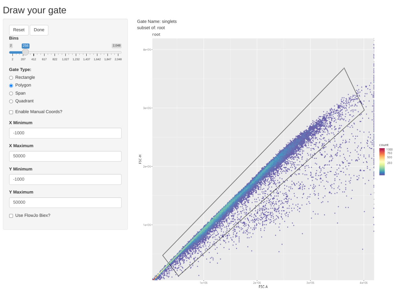
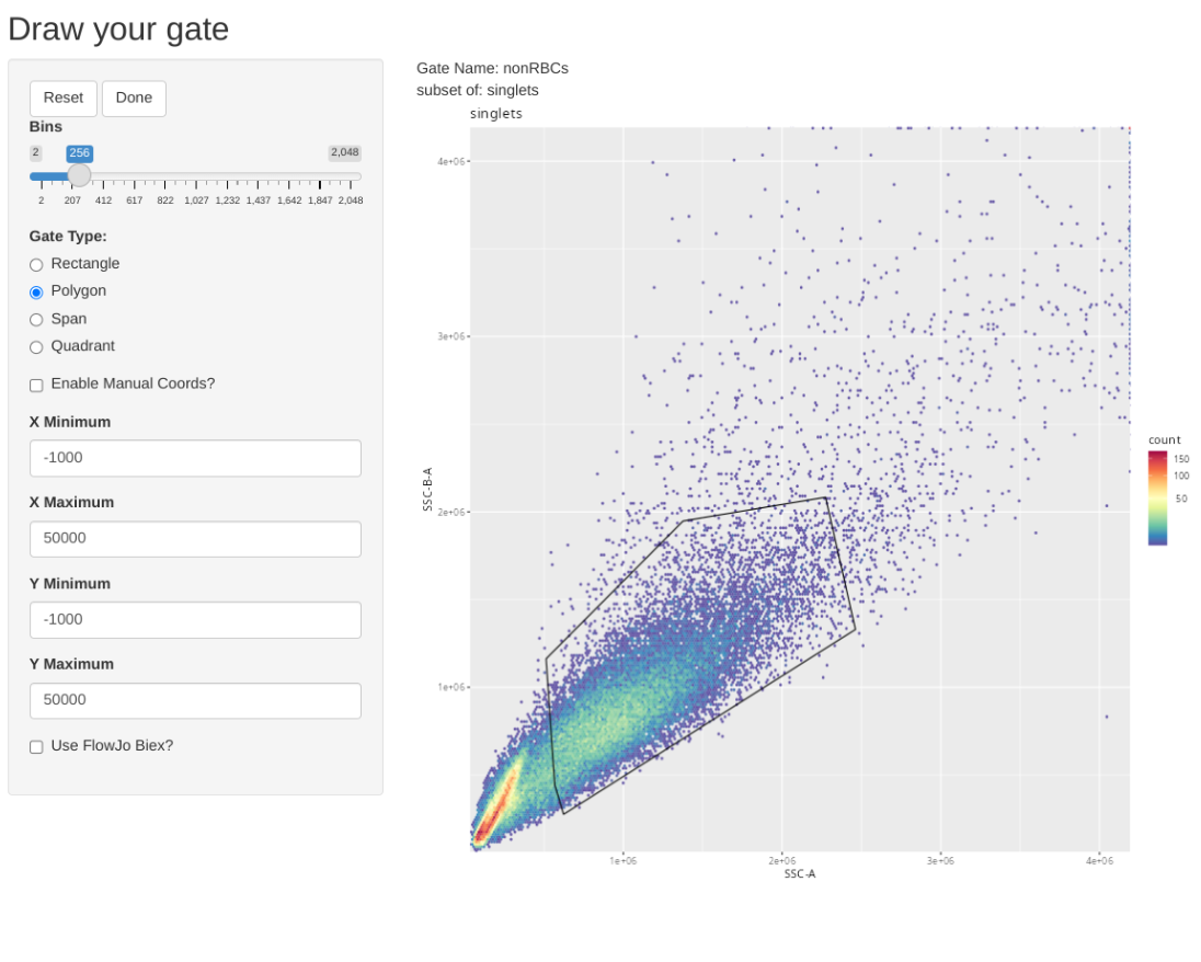
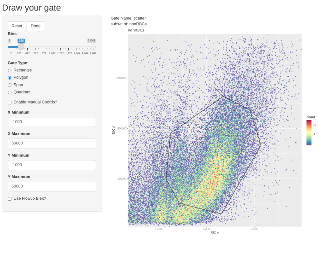
Consequently we will first gate for singlets, non-RBCs and lymphocyte scatter. Once this has been accomplished, we will downsample for 17500 of the present cells, which will result in being just under the 5 MB limit when using 5-laser Cytek Aurora raw .fcs files.

As always, start by loading the required R packages via the library() call.

library(flowWorkspace)

As part of improvements to flowWorkspace, some behavior of
GatingSet objects has changed. For details, please read the section
titled "The cytoframe and cytoset classes" in the package vignette:

  vignette("flowWorkspace-Introduction", "flowWorkspace")

library(flowGate)

Loading required package: ggcyto

Loading required package: ggplot2

Loading required package: flowCore

Loading required package: ncdfFlow

Loading required package: BH

library(dplyr)

Attaching package: 'dplyr'

The following object is masked from 'package:ncdfFlow':

    filter

The following object is masked from 'package:flowCore':

    filter

The following objects are masked from 'package:stats':

    filter, lag

The following objects are masked from 'package:base':

    intersect, setdiff, setequal, union

library(purrr)

Next, activate the Downsampling() function that was created as part of Week 10 of the course.

RFolder <- file.path("course", "community", "TRU-OLS",  "R") # For Interactive
# RFolder <- file.path("R") # For Quarto Rendering
MyFunctions <- list.files(RFolder, full.names=TRUE)
purrr::walk(.x=MyFunctions, .f=source)

With this done, specify your input file.path and output file.paths

#StorageLocation <- file.path("course", "community", "TRU-OLS", "data")
StorageLocation <- file.path("data")

#OutputLocation <- file.path("course", "community", "TRU-OLS", "outputs")
OutputLocation <- file.path("outputs")

And proceed to load in the .fcs files to a GatingSet.

fcs_files <- list.files(StorageLocation, pattern=".fcs",
 full.names=TRUE, recursive=TRUE)

SFC_cytoset <- load_cytoset_from_fcs(fcs_files,
 truncate_max_range=FALSE, transformation=FALSE)
SFC_GatingSet <- GatingSet(SFC_cytoset)

As we will be working with raw .fcs files today, we do not need to transform. If we did need to, we would use the following code (modifying the arguments to match our own instrument settings).

SFC_Parameters <- colnames(SFC_GatingSet)
FluorophoresOnly <- SFC_Parameters[!stringr::str_detect(SFC_Parameters, "FSC|SSC|Time")]

Biexponential <- flowjo_biexp_trans(channelRange=4096, maxValue=262144,
     pos=4.5, neg=2, widthBasis=-750)
MyBiexTransform <- transformerList(FluorophoresOnly, Biexponential)
transform(SFC_GatingSet, MyBiexTransform)

Next, we will create gates using the flowGate package, as covered during Week 08, specifically via the iteration table.

GatingTable <- tibble::tribble(
  ~filterId,    ~dims,                          ~subset,      
  "singlets",   list("FSC-A", "FSC-H"),          "root",  
  "nonRBCs",     list("SSC-A", "SSC-B-A"),    "singlets",
  "scatter",    list("FSC-A", "SSC-A"),      "nonRBCs",  
)

We can then run the following line of code, and proceed to sequentially draw the gates via the ShinyApp

flowGate::gs_apply_gating_strategy(SFC_GatingSet, gating_strategy = GatingTable)

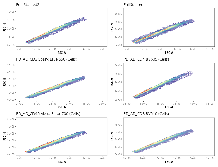
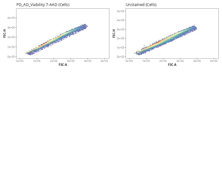
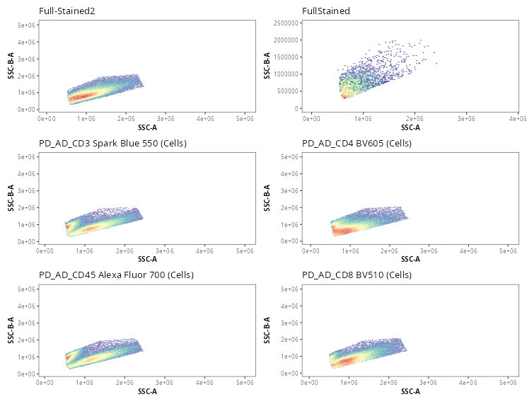
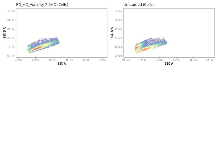
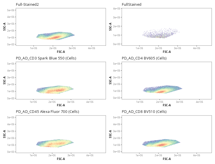
Once the gates are drawn, we can quickly validate that the gate placements will suffice for what we are trying to accomplish today. We can use the Utility_UnityPlots() from the Luciernaga package to compare the same gate across all specimens

library(Luciernaga)

Plot <- Utility_UnityPlot(x="FSC-A", y="FSC-H",
 GatingSet=SFC_GatingSet, sample.name="GUID", bins=70,
 removestrings=".fcs", marginsubset="root", gatesubset="singlets", returntype="patchwork", reference=NULL, clearance=0.2, gatelines=FALSE)

Plot2 <- Utility_UnityPlot(x="SSC-A", y="SSC-B-A",
 GatingSet=SFC_GatingSet, sample.name="GUID", bins=70,
 removestrings=".fcs", marginsubset="singlets", gatesubset="nonRBCs", returntype="patchwork", reference=NULL, clearance=0.2, gatelines=FALSE)

Plot3 <- Utility_UnityPlot(x="FSC-A", y="SSC-A",
 GatingSet=SFC_GatingSet, sample.name="GUID", bins=70,
 removestrings=".fcs", marginsubset="singlets", gatesubset="scatter", returntype="patchwork", reference=NULL, clearance=0.2, gatelines=FALSE)

With the gates reasonably enough placed (except for the Full-Stained 1 specimen), lets proceed and see what we have for counts.

Counts <- gs_pop_get_count_fast(SFC_GatingSet, "count")
Counts$Population <- basename(Counts$Population)
Counts |> filter(Population %in% "scatter")

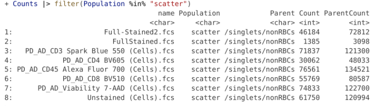
For a raw .fcs file from a 5-laser Cytek Aurora, downsampling to 17500 cells puts us just under the 5 MB limit. Seeing as we have enough cells, lets proceed to export out the downsampled .fcs files to our output folder.

purrr::walk(.x=SFC_GatingSet, subset="scatter", .f=Downsampling,
 DownsampleCount=17500, addon="scatter", returnType="fcs",
 StorageLocation=OutputLocation)

Proceeding

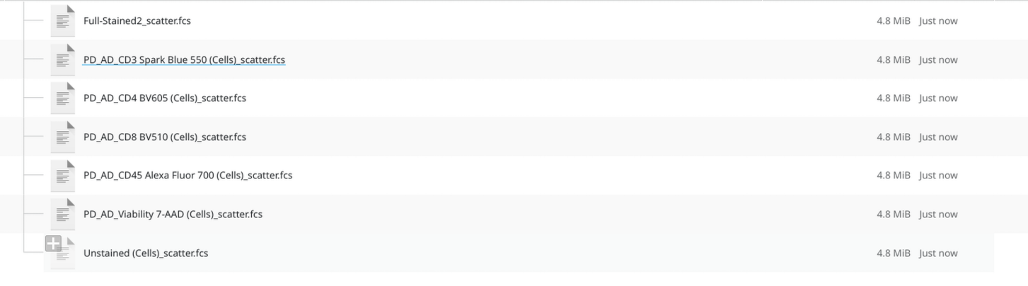
The resulting files are now under 5 MB. I proceeded to remove the original ones from the “data” folder, and replaced them with the files from the outputs folder. These were then transferred to GitHub for use in this walk-through example.

To return to where you were in the TRU-OLS walk-through, click here