12 - Spectral Signatures



For the YouTube livestream recording, see here
For screen-shot slides, click here
Background
.
Welcome back to the 12th week of the Cytometry in R course. For the next three session, we will be primarily focusing on topics related to spectral flow cytometry (SFC) (although they are also somewhat applicable to conventional flow cytometry (CFC)). In the process, we will continue to grow the functional programming skills we have been gradually accumulating through this middle section of the course.
.
When it comes to SFC, our ability to infer the presence or absence for particular fluorophores (as well as relative abundance) present on the surface of individual full-stained cells is directly tied to our ability to extract and provide reference fluorescent signatures from our unmixing controls (both single-color and unstained) that accurately match those same signatures as they are seen on the full-stained sample. These extracted fluorescent signatures are combined in the form of a matrix, which is referenced at the time of unmixing.
.
Over these next three sessions, my goal is that everyone gains hands-on-familiarity with the indiviudal steps in this process, so that what may currently seem to many as a black box is demystified. Additionally, the toolsets you’ll develop may help you find solutions and answer problems that we as a field are still grappling with.
.
While the focus of the primary course material is on providing context while building out skillsets, the bonus content accompanying these sessions is more geared towards showing how to implement the same topics as part of an everyday workflow.
Walk Through
Housekeeping
As we do every week, on GitHub, sync your forked version of the CytometryInR course to bring in the most recent updates. Then within Positron, pull in those changes to your local computer.
For YouTube walkthrough of this process, click here
After setting up a “Week12” project folder, copy over the contents of “course/12_SpectralSignatures/data” to that folder. This will hopefully prevent merge issues next week when attempting to pull in new course material. Once you have your new project folder organized, remember to commit and push your changes to GitHub to maintain remote version control.
If you encounter issues syncing due to the Take-Home Problem merge conflict, see this walkthrough. The updated homework submission protocol can be found here
Dataset
.
For this walk-through, we will be using the SDY3080 dataset from the NIH’s ImmPort repository. These .fcs files are the original data for our 2025 Cord Blood Innate-Like T cell paper, and is currently one of the few datasets on ImmPort that includes raw (i.e. not yet unmixed) .fcs files and the unmixing controls (single color and unstained), allowing for re-unmixing.
.
These .fcs files were acquired on a 5-laser Cytek Aurora (with 16 UV detectors, 16 Violet Detectors, 14 Blue Detectors, 10 Yellow-Green Detectors, and 8 Red detectors). Since raw .fcs files are substantially larger than their unmixed counterparts (due to the extra columns in the exprs matrix and all the associated metadata in parameters and keyword slots). Given GitHub file sharing limitations, after implementing clean-up gates, leftover events were downsampled for 5000 beads or 10000 cells as detailed in the bonus content.
.
For the .fcs files being used today, the unmixing controls consist of full sets of both bead and cell single-color controls. For the cell controls, these were composed of leftover Cord Blood Mononuclear Cells (CBMCs) or Peripheral Blood Mononuclear cells (PBMCs). There are additionally individual specimen unstained controls based on individual treatment conditions for background removal, and to isolate autofluorescence signatures for use in unmixing. Additional details can be found here.
.
If you want to follow along with your own spectral flow cytometry dataset, you can!!! In addition to the pre-processing steps we follow below, you may also want to check out the Bonus Material for additional details that have been abbreviated. One thing to be aware of, some of the reference control checking/visualization functions from Luciernaga haven’t been fully validated for non-Cytek instruments (as our core only has Cytek instruments, so no data to play around with during the original function creation). Please open a Discussion if you encounter issues/errors for something you suspect might be instrument keyword/column name related, as in most cases these are relatively simple fixes to implement.
Updating flowGate and Luciernaga
.
Over the “early summer” break, taking advantage of the open-source nature of the projects, I tackled some issues for both the flowGate and Luciernaga R packages, providing some additional useful functions to make the implementation of this walk-through easier. To take advantage of these changes, you will need to make sure to update both packages before continuing.
.
The easiest way to accomplish this would be to first uninstall these packages via the remove.packages() function
.
At which point, they can be reinstalled via the remotes package install_github() function.
.
At which point, we can check via packageVersion() to ensure we have at least the following versions installed.
Planning
.
As always with coding, it’s worthwhile to sketch out a brief plan of what you are trying to accomplish, breaking the overall task into smaller steps that can be tackled sequentially. It’s also worth thinking about what individual components are involved in the process when you are unmixing using commercial software as a point of comparison.
.
Since we are working in R with the .fcs files retrieved from ImmPort, we will need to load them into a GatingSet object similar to what we have been doing throughout the course. Likewise, since dead cells, debris, doublets may have different autofluorescence (or be especially prone to non-specific staining), we will likely need to implement some gates using flowGate to isolate just the cell or bead population we are interested in.
.
Once these initial clean-up gates are implemented, we will need to draw a gate around events “positive” for a given fluorophore, ideally those that are staining as bright or brighter in terms of MFI (meaning that on the x-axis of our plot we will need to correctly select the corresponding peak detector).
.
Once this is done, we can retrieve the exprs() matrix for those cells within the designated gate. We can then take the median/mean for each detector, followed by subtraction of the background to derive the values corresponding to the fluorophore. These are then typically normalized (scaled) so that all values range from 0 to 1. At this point, we will then need to visualize the normalized fluorescent signature to make sure we did everything correctly (or at least is reasonably accurate vs. published references).
.
At which point, we can repeat the process for…. however many fluorophores are in the SFC panel … (don’t worry, we will take advantage of somebody else’s functions to make this part less painful for those with medium or large panels).
Set Up
.
Alright, let’s go ahead and get our .fcs files into their GatingSet(s) and get some clean-up gates implemented. Fortunately for us, we can repurpose code that we have run previously, just repurposing it for this particular walk-through.
Loading R packages
.
Lets go ahead attach the R packages that we will need today to our local environment via the library() call, which makes the functions that each package contains available for our later use.
.
Next, lets create the variable/object containing the file.path to both today’s dataset, as well as an output storage location where we can store any intermediate outputs or plots.
.
With the file.path designated, lets check and see what .fcs files are currently present in our folder.
 [1] "data/DTR_2023_ILT_00-Reference Group-4BeadsUnstained (Beads).1237095.fcs"
 [2] "data/DTR_2023_ILT_00-Reference Group-DR_CCR4 BUV615 (Beads).1237096.fcs"
 [3] "data/DTR_2023_ILT_00-Reference Group-DR_CCR6 BV786 (Beads).1237097.fcs"
 [4] "data/DTR_2023_ILT_00-Reference Group-DR_CCR7 BV650 (Beads).1237098.fcs"
 [5] "data/DTR_2023_ILT_00-Reference Group-DR_CD107a APC-R700 (Beads).1237099.fcs"
 [6] "data/DTR_2023_ILT_00-Reference Group-DR_CD127 BV421 (Beads).1237100.fcs"
 [7] "data/DTR_2023_ILT_00-Reference Group-DR_CD16 APC (Beads).1237101.fcs"
 [8] "data/DTR_2023_ILT_00-Reference Group-DR_CD161 BV480 (Beads).1237102.fcs"
 [9] "data/DTR_2023_ILT_00-Reference Group-DR_CD25 PE-Cy5 (Beads).1237103.fcs"
[10] "data/DTR_2023_ILT_00-Reference Group-DR_CD26 PerCP-Cy5.5 (Beads).1237104.fcs"
[11] "data/DTR_2023_ILT_00-Reference Group-DR_CD27 APC-Fire 750 (Beads).1237105.fcs"
[12] "data/DTR_2023_ILT_00-Reference Group-DR_CD3 Alexa Fluor 488 (Beads).1237106.fcs"
[13] "data/DTR_2023_ILT_00-Reference Group-DR_CD3 Alexa Fluor 647 (Beads).1237107.fcs"
[14] "data/DTR_2023_ILT_00-Reference Group-DR_CD3 FITC (Beads).1237108.fcs"
[15] "data/DTR_2023_ILT_00-Reference Group-DR_CD3 Spark Blue 550 (Beads).1237109.fcs"
[16] "data/DTR_2023_ILT_00-Reference Group-DR_CD38 APC-Fire 810 (Beads).1237110.fcs"
[17] "data/DTR_2023_ILT_00-Reference Group-DR_CD4 BUV805 (Beads).1237111.fcs"
[18] "data/DTR_2023_ILT_00-Reference Group-DR_CD45RA BV510 (Beads).1237112.fcs"
[19] "data/DTR_2023_ILT_00-Reference Group-DR_CD56 BV605 (Beads).1237113.fcs"
[20] "data/DTR_2023_ILT_00-Reference Group-DR_CD62L BUV395 (Beads).1237114.fcs"
[21] "data/DTR_2023_ILT_00-Reference Group-DR_CD69 BUV563 (Beads).1237115.fcs"
[22] "data/DTR_2023_ILT_00-Reference Group-DR_CD7 BV711 (Beads).1237116.fcs"
[23] "data/DTR_2023_ILT_00-Reference Group-DR_CD8 BUV496 (Beads).1237117.fcs"
[24] "data/DTR_2023_ILT_00-Reference Group-DR_CXCR3 BUV737 (Beads).1237118.fcs"
[25] "data/DTR_2023_ILT_00-Reference Group-DR_Dump_CD14 Pacific Blue (Beads).1237119.fcs"
[26] "data/DTR_2023_ILT_00-Reference Group-DR_Dump_CD19 Pacific Blue (Beads).1237120.fcs"
[27] "data/DTR_2023_ILT_00-Reference Group-DR_IFNg BV750 (Beads).1237121.fcs"
[28] "data/DTR_2023_ILT_00-Reference Group-DR_NKG2D PE (Beads).1237122.fcs"
[29] "data/DTR_2023_ILT_00-Reference Group-DR_PD1 PE-Vio770 (Beads).1237123.fcs"
[30] "data/DTR_2023_ILT_00-Reference Group-DR_TNFa PE-Dazzle594 (Beads).1237124.fcs"
[31] "data/DTR_2023_ILT_00-Reference Group-DR_Va24Ja18 FITC (Beads).1237125.fcs"
[32] "data/DTR_2023_ILT_00-Reference Group-DR_Va7.2 Alexa Fluor 647 (Beads).1237126.fcs"
[33] "data/DTR_2023_ILT_00-Reference Group-DR_VD2 BUV661 (Beads).1237127.fcs"
[34] "data/DTR_2023_ILT_01-INF052-Ctrl_Unstained.1235650.fcs"
[35] "data/DTR_2023_ILT_01-ND006_v1-Ctrl_Unstained.1235671.fcs"
[36] "data/DTR_2023_ILT_01-ND006_v1-PMA_Unstained.1235672.fcs"
[37] "data/DTR_2023_ILT_01-Reference Group-DR_CCR4 BUV615 (Cells).1235678.fcs"
[38] "data/DTR_2023_ILT_01-Reference Group-DR_CCR6 BV786 (Cells).1235679.fcs"
[39] "data/DTR_2023_ILT_01-Reference Group-DR_CCR7 BV650 (Cells).1235680.fcs"
[40] "data/DTR_2023_ILT_01-Reference Group-DR_CD107a APC-R700 (Cells).1235681.fcs"
[41] "data/DTR_2023_ILT_01-Reference Group-DR_CD127 BV421 (Cells).1235682.fcs"
[42] "data/DTR_2023_ILT_01-Reference Group-DR_CD16 APC (Cells).1235683.fcs"
[43] "data/DTR_2023_ILT_01-Reference Group-DR_CD161 BV480 (Cells).1235684.fcs"
[44] "data/DTR_2023_ILT_01-Reference Group-DR_CD25 PE-Cy5 (Cells).1235685.fcs"
[45] "data/DTR_2023_ILT_01-Reference Group-DR_CD26 PerCP-Cy5.5 (Cells).1235686.fcs"
[46] "data/DTR_2023_ILT_01-Reference Group-DR_CD27 APC-Fire 750 (Cells).1235687.fcs"
[47] "data/DTR_2023_ILT_01-Reference Group-DR_CD3 Alexa Fluor 488 (Cells).1235688.fcs"
[48] "data/DTR_2023_ILT_01-Reference Group-DR_CD3 Alexa Fluor 647 (Cells).1235689.fcs"
[49] "data/DTR_2023_ILT_01-Reference Group-DR_CD3 FITC (Cells).1235690.fcs"
[50] "data/DTR_2023_ILT_01-Reference Group-DR_CD3 Spark Blue 550 (Cells).1235691.fcs"
[51] "data/DTR_2023_ILT_01-Reference Group-DR_CD38 APC-Fire 810 (Cells).1235692.fcs"
[52] "data/DTR_2023_ILT_01-Reference Group-DR_CD4 BUV805 (Cells).1235693.fcs"
[53] "data/DTR_2023_ILT_01-Reference Group-DR_CD45RA BV510 (Cells).1235694.fcs"
[54] "data/DTR_2023_ILT_01-Reference Group-DR_CD56 BV605 (Cells).1235695.fcs"
[55] "data/DTR_2023_ILT_01-Reference Group-DR_CD62L BUV395 (Cells).1235696.fcs"
[56] "data/DTR_2023_ILT_01-Reference Group-DR_CD69 BUV563 (Cells).1235697.fcs"
[57] "data/DTR_2023_ILT_01-Reference Group-DR_CD7 BV711 (Cells).1235698.fcs"
[58] "data/DTR_2023_ILT_01-Reference Group-DR_CD8 BUV496 (Cells).1235699.fcs"
[59] "data/DTR_2023_ILT_01-Reference Group-DR_CXCR3 BUV737 (Cells).1235700.fcs"
[60] "data/DTR_2023_ILT_01-Reference Group-DR_Dump_CD14 Pacific Blue (Cells).1235701.fcs"
[61] "data/DTR_2023_ILT_01-Reference Group-DR_Dump_CD19 Pacific Blue (Cells).1235702.fcs"
[62] "data/DTR_2023_ILT_01-Reference Group-DR_IFNg BV750 (Cells).1235703.fcs"
[63] "data/DTR_2023_ILT_01-Reference Group-DR_NKG2D PE (Cells).1235704.fcs"
[64] "data/DTR_2023_ILT_01-Reference Group-DR_PD1 PE-Vio770 (Cells).1235705.fcs"
[65] "data/DTR_2023_ILT_01-Reference Group-DR_TNFa PE-Dazzle594 (Cells).1235706.fcs"
[66] "data/DTR_2023_ILT_01-Reference Group-DR_VD2 BUV661 (Cells).1235707.fcs"
[67] "data/DTR_2023_ILT_01-Reference Group-DR_Viability Zombie NIR (Cells).1235708.fcs"
[68] "data/DTR_2023_ILT_01-Reference Group-DR_Viability_PMA Zombie NIR (Cells).1235709.fcs"
.
Looking at the file names, we need to figure out a way to separate the bead single-color controls from the cell single-color controls and cell unstained controls.
.
As we glance through, it appears that the bead unmixing controls all share the “ILT_00” and “(Beads)” character strings in their file names, while all cell unmixing controls contain “ILT_01” and “(Cells)” character strings in their file name.
.
Additionally, there are 3 cell unstained controls that are designated by the presence of “_Unstained”.
.
Using the stringr package, we can utilize str_detect() function within the square brackets to subset the original vector list just for those files that match the search pattern (i.e. those returning as TRUE). In combination, this results in separate vector lists for the different unmixing control types
 [1] "data/DTR_2023_ILT_00-Reference Group-4BeadsUnstained (Beads).1237095.fcs"
 [2] "data/DTR_2023_ILT_00-Reference Group-DR_CCR4 BUV615 (Beads).1237096.fcs"
 [3] "data/DTR_2023_ILT_00-Reference Group-DR_CCR6 BV786 (Beads).1237097.fcs"
 [4] "data/DTR_2023_ILT_00-Reference Group-DR_CCR7 BV650 (Beads).1237098.fcs"
 [5] "data/DTR_2023_ILT_00-Reference Group-DR_CD107a APC-R700 (Beads).1237099.fcs"
 [6] "data/DTR_2023_ILT_00-Reference Group-DR_CD127 BV421 (Beads).1237100.fcs"
 [7] "data/DTR_2023_ILT_00-Reference Group-DR_CD16 APC (Beads).1237101.fcs"
 [8] "data/DTR_2023_ILT_00-Reference Group-DR_CD161 BV480 (Beads).1237102.fcs"
 [9] "data/DTR_2023_ILT_00-Reference Group-DR_CD25 PE-Cy5 (Beads).1237103.fcs"
[10] "data/DTR_2023_ILT_00-Reference Group-DR_CD26 PerCP-Cy5.5 (Beads).1237104.fcs"
[11] "data/DTR_2023_ILT_00-Reference Group-DR_CD27 APC-Fire 750 (Beads).1237105.fcs"
[12] "data/DTR_2023_ILT_00-Reference Group-DR_CD3 Alexa Fluor 488 (Beads).1237106.fcs"
[13] "data/DTR_2023_ILT_00-Reference Group-DR_CD3 Alexa Fluor 647 (Beads).1237107.fcs"
[14] "data/DTR_2023_ILT_00-Reference Group-DR_CD3 FITC (Beads).1237108.fcs"
[15] "data/DTR_2023_ILT_00-Reference Group-DR_CD3 Spark Blue 550 (Beads).1237109.fcs"
[16] "data/DTR_2023_ILT_00-Reference Group-DR_CD38 APC-Fire 810 (Beads).1237110.fcs"
[17] "data/DTR_2023_ILT_00-Reference Group-DR_CD4 BUV805 (Beads).1237111.fcs"
[18] "data/DTR_2023_ILT_00-Reference Group-DR_CD45RA BV510 (Beads).1237112.fcs"
[19] "data/DTR_2023_ILT_00-Reference Group-DR_CD56 BV605 (Beads).1237113.fcs"
[20] "data/DTR_2023_ILT_00-Reference Group-DR_CD62L BUV395 (Beads).1237114.fcs"
[21] "data/DTR_2023_ILT_00-Reference Group-DR_CD69 BUV563 (Beads).1237115.fcs"
[22] "data/DTR_2023_ILT_00-Reference Group-DR_CD7 BV711 (Beads).1237116.fcs"
[23] "data/DTR_2023_ILT_00-Reference Group-DR_CD8 BUV496 (Beads).1237117.fcs"
[24] "data/DTR_2023_ILT_00-Reference Group-DR_CXCR3 BUV737 (Beads).1237118.fcs"
[25] "data/DTR_2023_ILT_00-Reference Group-DR_Dump_CD14 Pacific Blue (Beads).1237119.fcs"
[26] "data/DTR_2023_ILT_00-Reference Group-DR_Dump_CD19 Pacific Blue (Beads).1237120.fcs"
[27] "data/DTR_2023_ILT_00-Reference Group-DR_IFNg BV750 (Beads).1237121.fcs"
[28] "data/DTR_2023_ILT_00-Reference Group-DR_NKG2D PE (Beads).1237122.fcs"
[29] "data/DTR_2023_ILT_00-Reference Group-DR_PD1 PE-Vio770 (Beads).1237123.fcs"
[30] "data/DTR_2023_ILT_00-Reference Group-DR_TNFa PE-Dazzle594 (Beads).1237124.fcs"
[31] "data/DTR_2023_ILT_00-Reference Group-DR_Va24Ja18 FITC (Beads).1237125.fcs"
[32] "data/DTR_2023_ILT_00-Reference Group-DR_Va7.2 Alexa Fluor 647 (Beads).1237126.fcs"
[33] "data/DTR_2023_ILT_00-Reference Group-DR_VD2 BUV661 (Beads).1237127.fcs" [1] "data/DTR_2023_ILT_01-Reference Group-DR_CCR4 BUV615 (Cells).1235678.fcs"
[2] "data/DTR_2023_ILT_01-Reference Group-DR_CCR6 BV786 (Cells).1235679.fcs"
[3] "data/DTR_2023_ILT_01-Reference Group-DR_CCR7 BV650 (Cells).1235680.fcs"
[4] "data/DTR_2023_ILT_01-Reference Group-DR_CD107a APC-R700 (Cells).1235681.fcs"
[5] "data/DTR_2023_ILT_01-Reference Group-DR_CD127 BV421 (Cells).1235682.fcs"
[6] "data/DTR_2023_ILT_01-Reference Group-DR_CD16 APC (Cells).1235683.fcs"
[7] "data/DTR_2023_ILT_01-Reference Group-DR_CD161 BV480 (Cells).1235684.fcs"
[8] "data/DTR_2023_ILT_01-Reference Group-DR_CD25 PE-Cy5 (Cells).1235685.fcs"
[9] "data/DTR_2023_ILT_01-Reference Group-DR_CD26 PerCP-Cy5.5 (Cells).1235686.fcs"
[10] "data/DTR_2023_ILT_01-Reference Group-DR_CD27 APC-Fire 750 (Cells).1235687.fcs"
[11] "data/DTR_2023_ILT_01-Reference Group-DR_CD3 Alexa Fluor 488 (Cells).1235688.fcs"
[12] "data/DTR_2023_ILT_01-Reference Group-DR_CD3 Alexa Fluor 647 (Cells).1235689.fcs"
[13] "data/DTR_2023_ILT_01-Reference Group-DR_CD3 FITC (Cells).1235690.fcs"
[14] "data/DTR_2023_ILT_01-Reference Group-DR_CD3 Spark Blue 550 (Cells).1235691.fcs"
[15] "data/DTR_2023_ILT_01-Reference Group-DR_CD38 APC-Fire 810 (Cells).1235692.fcs"
[16] "data/DTR_2023_ILT_01-Reference Group-DR_CD4 BUV805 (Cells).1235693.fcs"
[17] "data/DTR_2023_ILT_01-Reference Group-DR_CD45RA BV510 (Cells).1235694.fcs"
[18] "data/DTR_2023_ILT_01-Reference Group-DR_CD56 BV605 (Cells).1235695.fcs"
[19] "data/DTR_2023_ILT_01-Reference Group-DR_CD62L BUV395 (Cells).1235696.fcs"
[20] "data/DTR_2023_ILT_01-Reference Group-DR_CD69 BUV563 (Cells).1235697.fcs"
[21] "data/DTR_2023_ILT_01-Reference Group-DR_CD7 BV711 (Cells).1235698.fcs"
[22] "data/DTR_2023_ILT_01-Reference Group-DR_CD8 BUV496 (Cells).1235699.fcs"
[23] "data/DTR_2023_ILT_01-Reference Group-DR_CXCR3 BUV737 (Cells).1235700.fcs"
[24] "data/DTR_2023_ILT_01-Reference Group-DR_Dump_CD14 Pacific Blue (Cells).1235701.fcs"
[25] "data/DTR_2023_ILT_01-Reference Group-DR_Dump_CD19 Pacific Blue (Cells).1235702.fcs"
[26] "data/DTR_2023_ILT_01-Reference Group-DR_IFNg BV750 (Cells).1235703.fcs"
[27] "data/DTR_2023_ILT_01-Reference Group-DR_NKG2D PE (Cells).1235704.fcs"
[28] "data/DTR_2023_ILT_01-Reference Group-DR_PD1 PE-Vio770 (Cells).1235705.fcs"
[29] "data/DTR_2023_ILT_01-Reference Group-DR_TNFa PE-Dazzle594 (Cells).1235706.fcs"
[30] "data/DTR_2023_ILT_01-Reference Group-DR_VD2 BUV661 (Cells).1235707.fcs"
[31] "data/DTR_2023_ILT_01-Reference Group-DR_Viability Zombie NIR (Cells).1235708.fcs"
[32] "data/DTR_2023_ILT_01-Reference Group-DR_Viability_PMA Zombie NIR (Cells).1235709.fcs"Gating Sets
.
Now that we have separated out the individual .fcs files based on type of unmixing control, lets proceed to load each into their own GatingSets. This will make our lives a little bit easier in the long run, as we will only be working with 1 type of unmixing control per GatingSet when it comes time to iterate.
Beads_cytoset <- load_cytoset_from_fcs(Bead_FCS, truncate_max_range=FALSE, transformation=FALSE)
BeadsSC_GatingSet <- GatingSet(Beads_cytoset)


Cells_cytoset <- load_cytoset_from_fcs(Cell_FCS, truncate_max_range=FALSE, transformation=FALSE)
CellsSC_GatingSet <- GatingSet(Cells_cytoset)

UnstainedCells_cytoset <- load_cytoset_from_fcs(UnstainedCell_FCS, truncate_max_range=FALSE, transformation=FALSE)
CellsUnstained_GatingSet <- GatingSet(UnstainedCells_cytoset)
Should we Transform?
.
If you recall previous weeks, you may recall that normally at this point of the pre-processing, we transform our fluorescent detectors/parameters. Since our ultimate goal is to extract spectral fluorescent signature values from our raw .fcs files, you may be wondering if we need to transform at all (given that the transformation will change the underlying values, which depending on the parameters/arguments given may bias the shape of the signature). This intuition is a good one, as this is something we indeed want to avoid.
.
However, between our current point (assembled GatingSet) and then (extracting exprs), we still need to create a positive gate on the events that are bright or brighter for the given fluorophore’s peak detector. Since fluorescent values tend to be spread out on a biexponential scale, doing this without transforming can be challenging.
.
Consequently, it’s easier for our workflow if we go ahead and transform first, gate, and then remember to set the “inverse.transform = TRUE” argument at the time of cytoset/exprs extraction to ensure we are getting the original raw values. Lets therefore go ahead and apply transformations for our fluorescent detectors channels.
# Identify biexponential fluorescent detectors, exclude linear ones like FSC

SFC_Parameters <- colnames(CellsUnstained_GatingSet)
FluorophoresOnly <- SFC_Parameters[!stringr::str_detect(SFC_Parameters, "FSC|SSC|Time")]

# Biexponential values that were optimal for this particular instrument/dataset, yours may vary, see Week 7!

Biexponential <-  flowjo_biexp_trans(channelRange=4096, maxValue=4194304,
  pos=5.62, neg=0, widthBasis=-1000)
MyBiexTransform <- transformerList(FluorophoresOnly, Biexponential)

# Beads Single Colors

transform(BeadsSC_GatingSet, MyBiexTransform)
A GatingSet with 33 samplesA GatingSet with 32 samplesA GatingSet with 3 samplesClean Up Gates
.
For our clean-up gates, we have a couple methods by which we can implement them. Lets go with the manual method via the flowGate package’s Shiny app for now, which in turn will allow us to see the functionality of the new functions that were added to it.
.
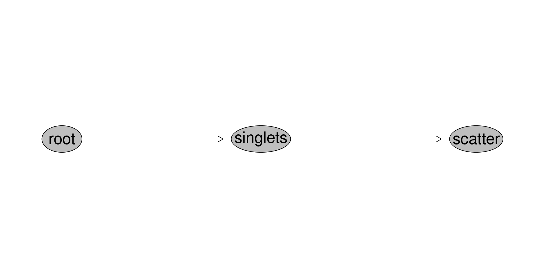
Lets set up a GatingTable template for the gates we want to create (scatter and singlets for the bead controls, singlets and scatter for the cell controls)
BeadGatingTable <- tibble::tribble(
  ~filterId,    ~dims,                          ~subset,
  "scatter",    list("FSC-A", "SSC-A"),      "root",
  "singlets",   list("FSC-A", "FSC-H"),          "scatter"
)


CellGatingTable <- tibble::tribble(
  ~filterId,    ~dims,                          ~subset,
  "singlets",   list("FSC-A", "FSC-H"),          "root",
  "scatter",    list("FSC-A", "SSC-A"),      "singlets",
)
Beads Single Colors
.
With the GatingTables defined, we can then use the gs_apply_gating_strategy() function and iterate through the gate drawing, similar to what we have already encountered back during Week 08
.
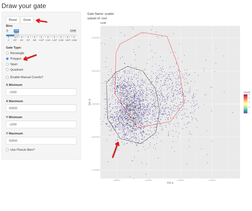
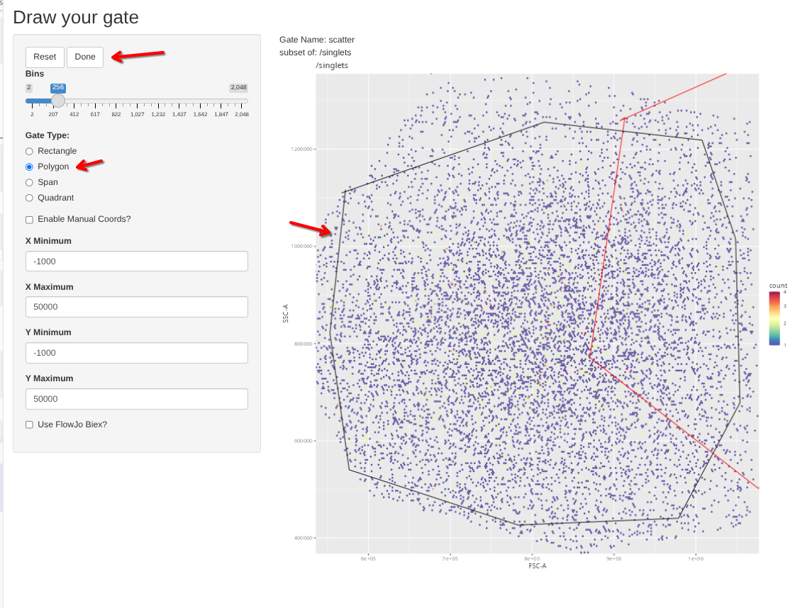
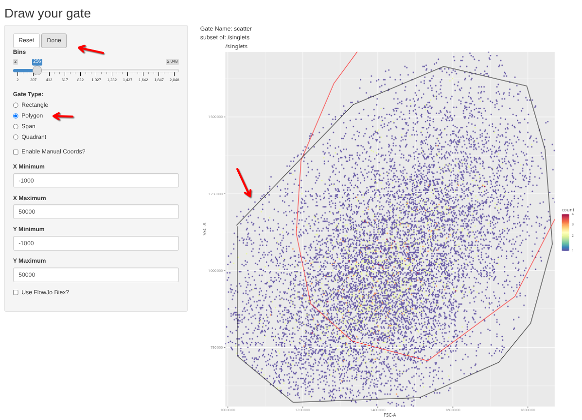
Once the ShinyApp launches, select polygon, draw your gate based on scatter, and click Done. If you mess us, hit reset. Remember, these particular example files were “pre-cleaned” and “downsampled”, so ggplot2 has a tendency to zoom in.
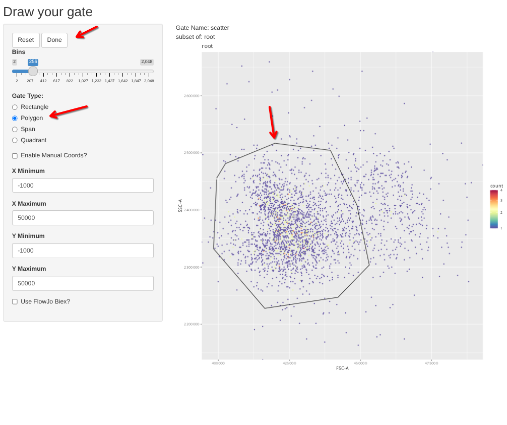
And next, draw your scatter gate.
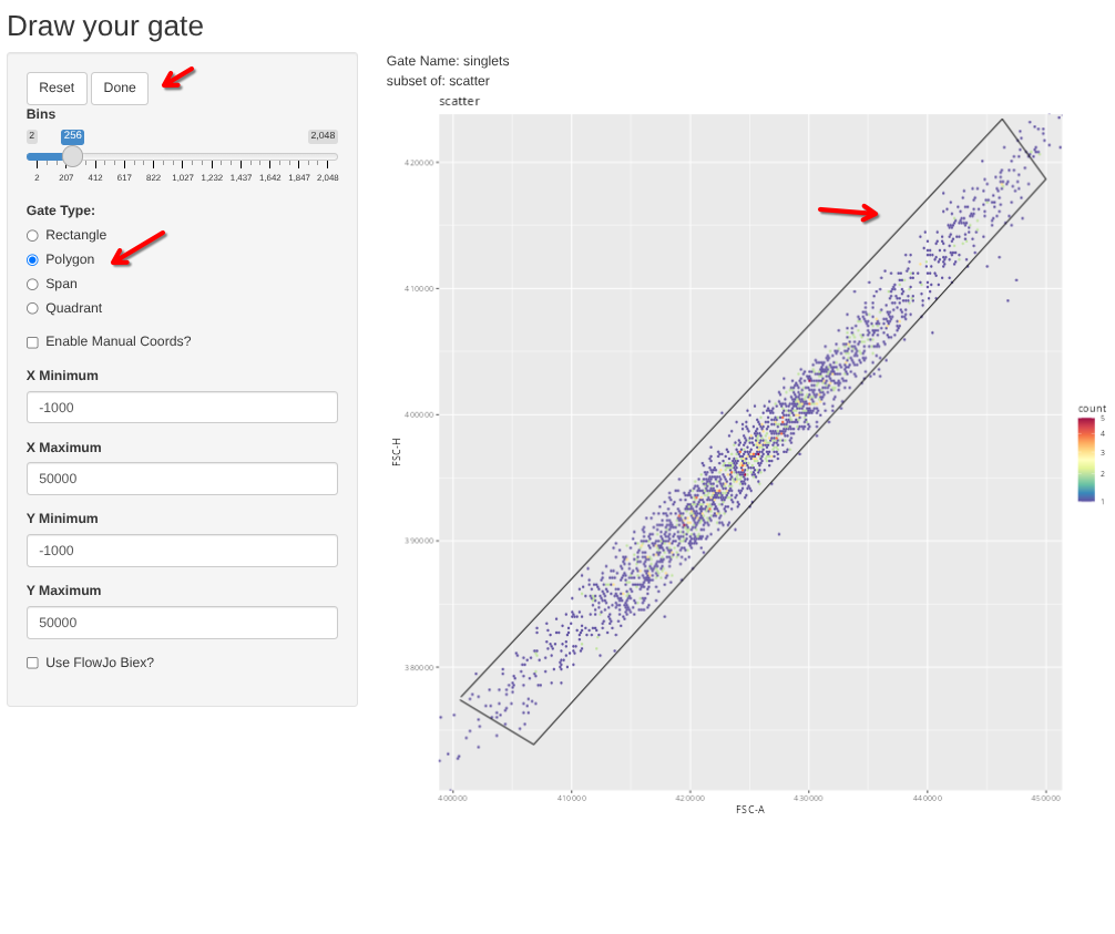
.
Now that these initial gates have been applied to our GatingSet, we need to evaluate whether they were applied correctly for each individual specimen. In the old version of flowGate, this was a one-size-fits-all, and if it was off, we would need to recreate the gate across the board to try to account for this.
.
Since the ability to change the gate position for an individual specimen was already present in the flowWorkspace package, the new gs_apply_gate_check() function in flowGate takes advantage of this functionality by iterating through individual specimens in a GatingSet, allowing adjustments to be made for that specific gate on an individual basis.
.
If for a given specimen the gate is good as is, just select “Done”.
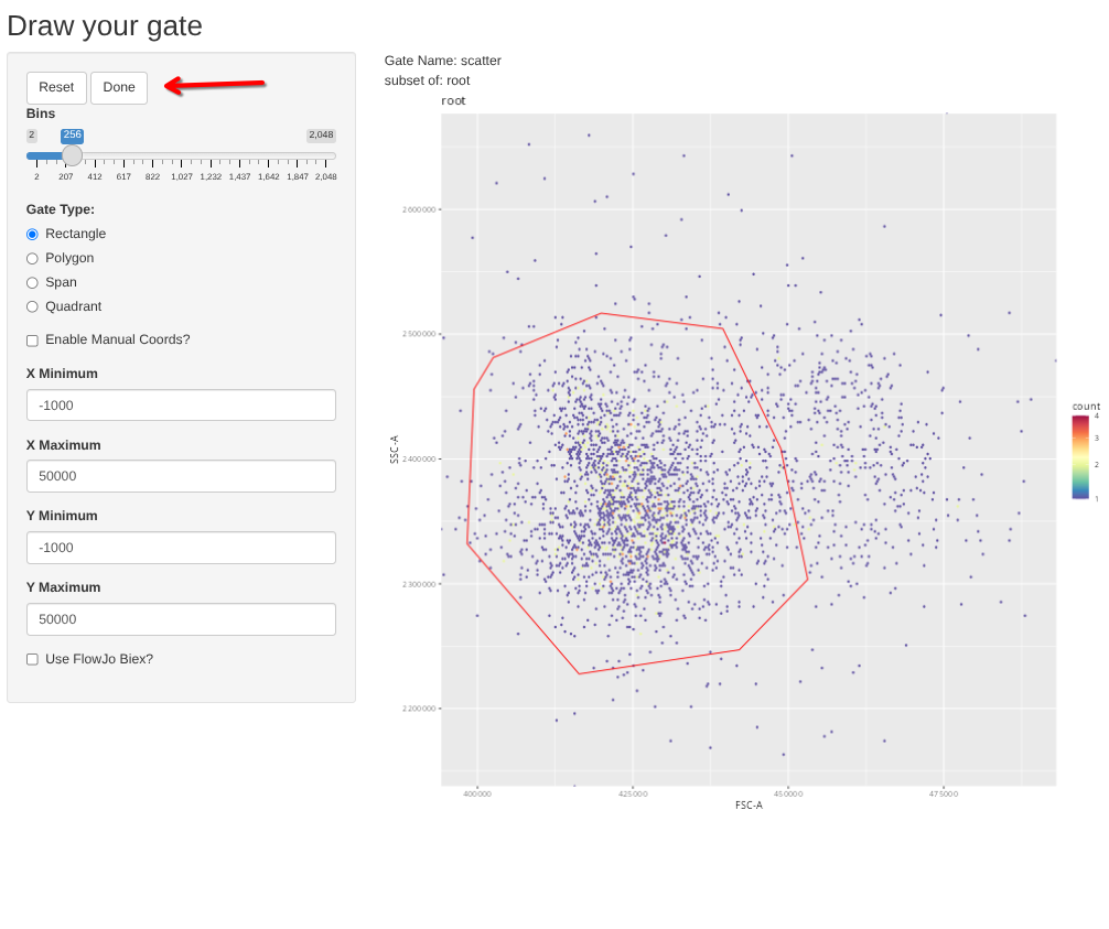
.
If it needs changing, draw a better polygon gate, and then select “Done”. Here are a couple examples where different adjustments were made.
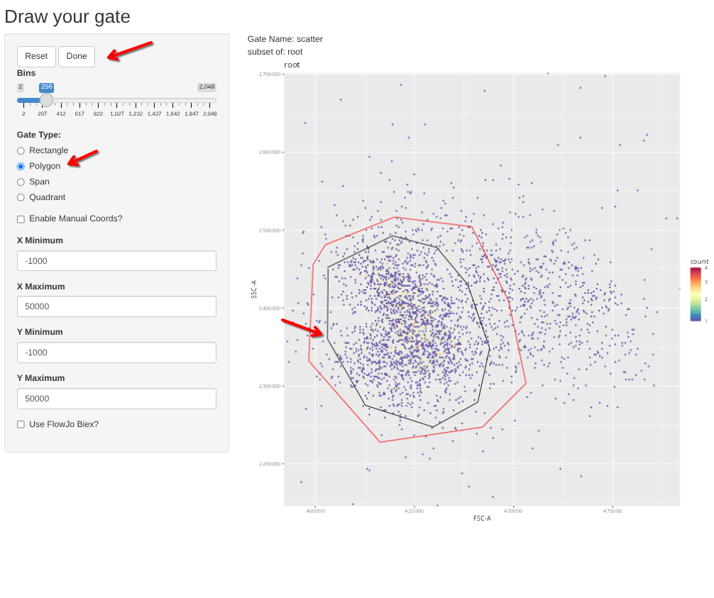
.
With this first gate (“scatter”) now checked across all specimens, we just need to repeat the process for the other applied gate (“singlets”).
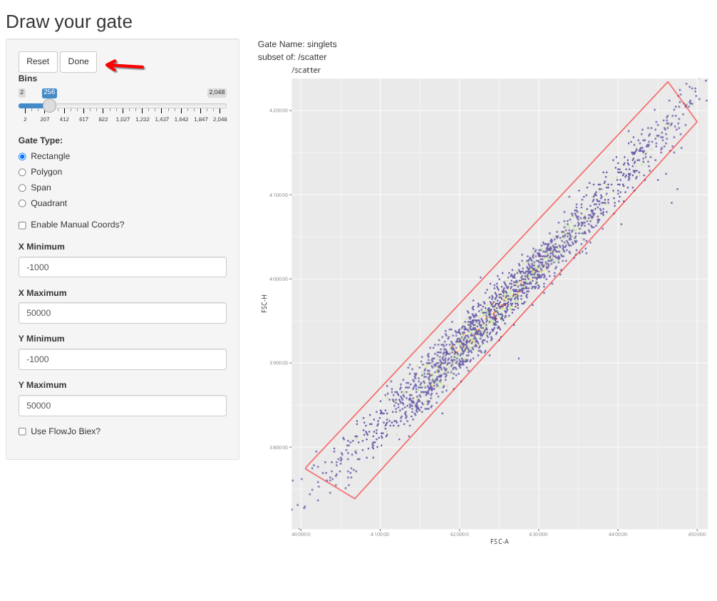
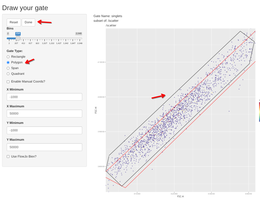
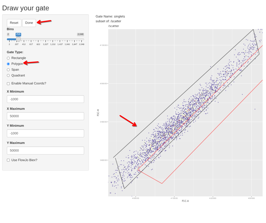
.
And with that, the Bead Single-Color controls have been properly gated. On to the next unmixing control type!
Cells Single Colors
.
At this point, we can repeat the process for our Cell Single Color controls, first applying initial gates to the GatingSet via gs_apply_gating_strategy()
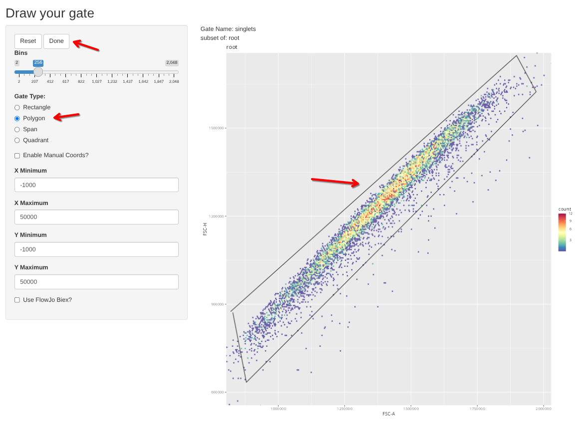
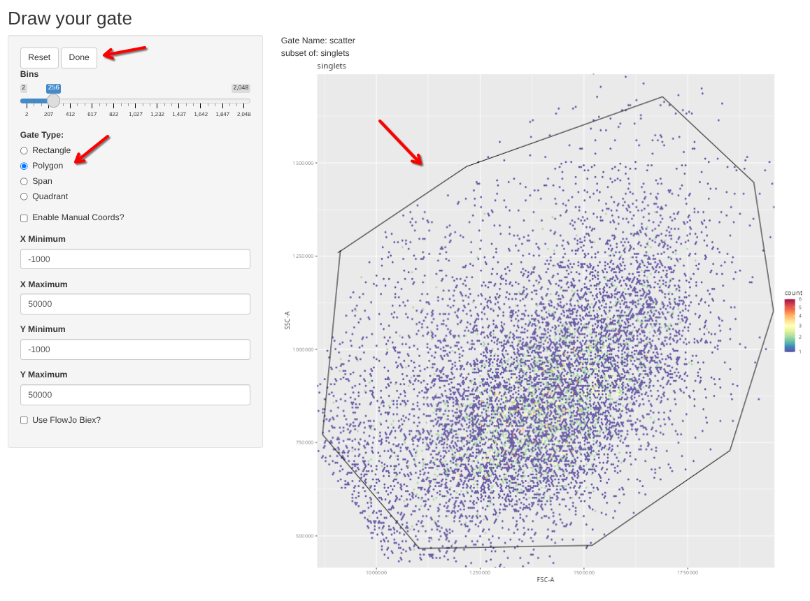
.
And then checking/editing the individual gates across individual specimens via gs_apply_gate_check().
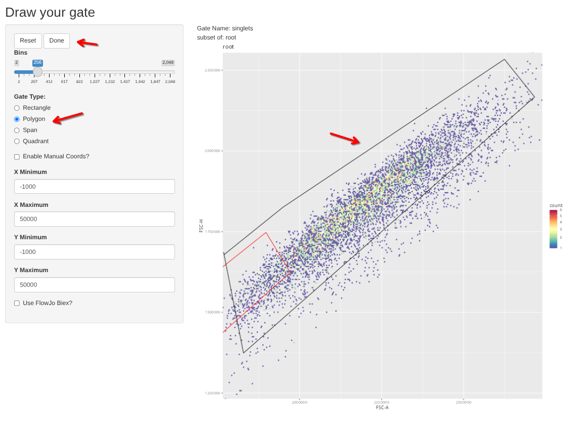
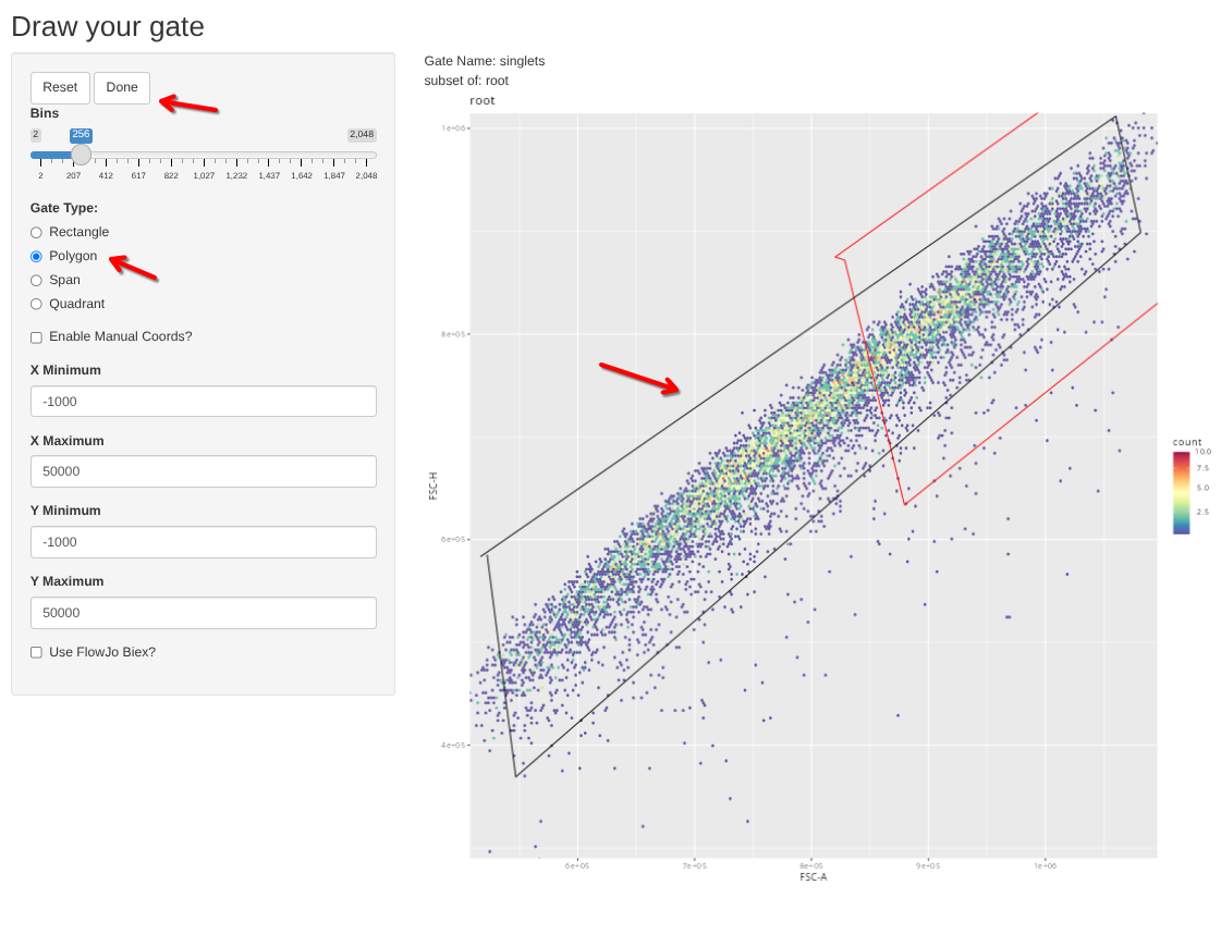
.
And with that, the cell single-color controls are also now correctly gated for each gate at the individual level.
Cells Unstained
.
And last (but definitely not least), lets repeat the process for our cell unstained controls. Lets apply gates via gs_apply_gating_strategy()
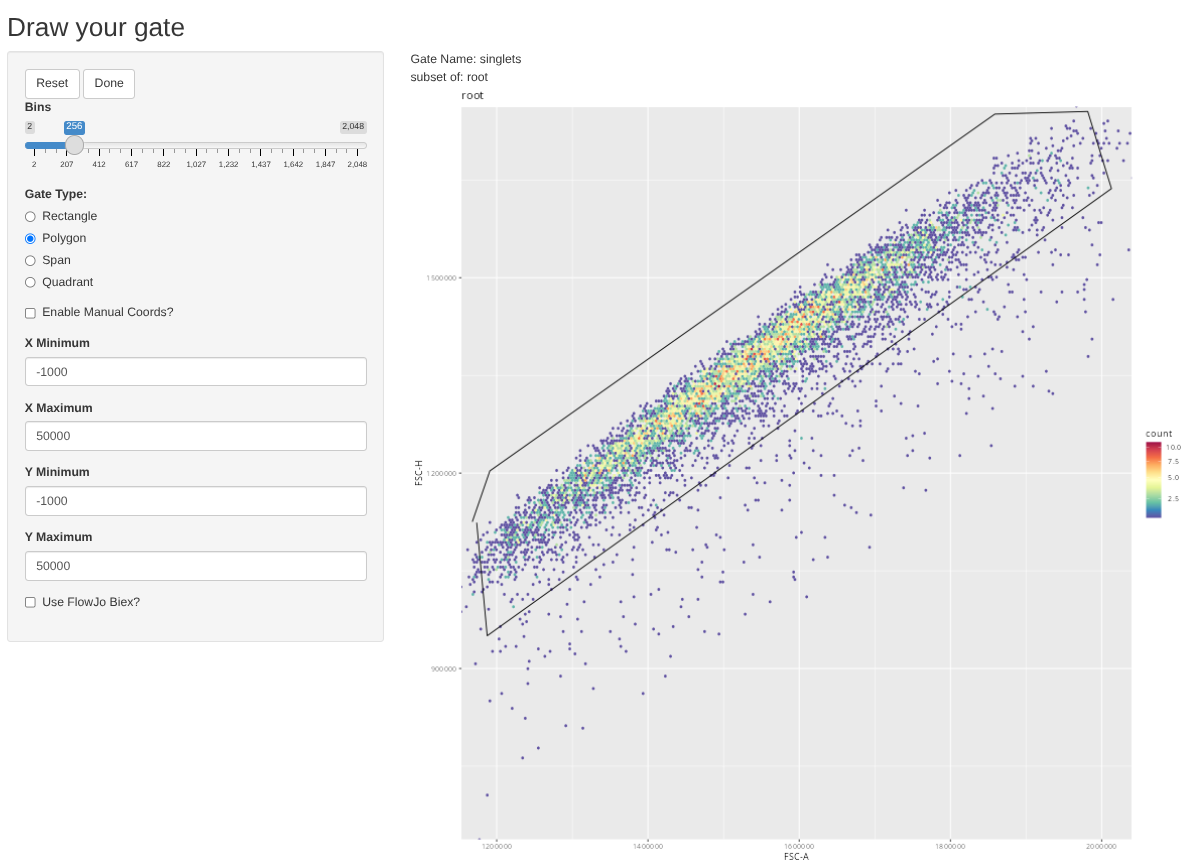
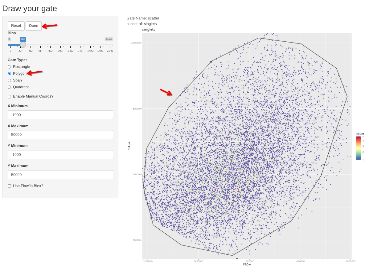
.
And check the positioning of the individual gates via gs_apply_gate_check(), modifying as needed.
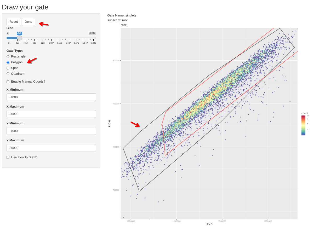
.
And hurray! All gates have been applied correctly for all our unmixing controls across their respective GatingSets.
Metadata
.
With the clean-up gates implemented, lets wrap up the set up process by adding some additional metadata columns. This will make subsetting the GatingSet for individual unmixing controls easier to implement later today.
.
Currently, the only column in metadata is the name column, containing the long filename we saw in the file paths above.
.
However, within this filename we also have information related to the antigen, fluorophore, and control type (beads or cells). Since Regular Expressions (RegEx) is not generally people’s forte, we can ask an LLM to provide us the correct syntax (see example within str_extract() next to “name”) needed to extract these bits of information from the current filenames, and integrate this as new columns in concert with the dplyr packages mutate() and case_when() functions, as well as some of string clean-up functions from the stringr package.
Beads Single Colors
.
Lets start first with the single-color beads, and see if the LLM gave us the correct RegEx pattern, or just hallucinated garbage.
bead_pd <- pData(BeadsSC_GatingSet)

Updated_bead_pd <- bead_pd |> mutate(
    raw = str_extract(name, "(?<=DR_)[^(]+(?=\\()"),
    Antigen = raw |>
      str_trim() |>
      str_extract("^\\S+"),
    Fluorophore = raw |>
      str_trim() |>
      str_remove("^\\S+\\s+"),
    Type = name |>
      str_extract("(?<=\\()([^)]+)(?=\\))"),
    raw = NULL
  )

Updated_bead_pd <- Updated_bead_pd |> relocate(Fluorophore, Antigen, Type, .after="name") Fluorophore Antigen Type
1 <NA> <NA> Beads
2 BUV615 CCR4 Beads
3 BV786 CCR6 Beads
4 BV650 CCR7 Beads
5 APC-R700 CD107a Beads
6 BV421 CD127 Beads
7 APC CD16 Beads
8 BV480 CD161 Beads
9 PE-Cy5 CD25 Beads
10 PerCP-Cy5.5 CD26 Beads
11 APC-Fire 750 CD27 Beads
12 Alexa Fluor 488 CD3 Beads
13 Alexa Fluor 647 CD3 Beads
14 FITC CD3 Beads
15 Spark Blue 550 CD3 Beads
16 APC-Fire 810 CD38 Beads
17 BUV805 CD4 Beads
18 BV510 CD45RA Beads
19 BV605 CD56 Beads
20 BUV395 CD62L Beads
21 BUV563 CD69 Beads
22 BV711 CD7 Beads
23 BUV496 CD8 Beads
24 BUV737 CXCR3 Beads
25 Pacific Blue Dump_CD14 Beads
26 Pacific Blue Dump_CD19 Beads
27 BV750 IFNg Beads
28 PE NKG2D Beads
29 PE-Vio770 PD1 Beads
30 PE-Dazzle594 TNFa Beads
31 FITC Va24Ja18 Beads
32 Alexa Fluor 647 Va7.2 Beads
33 BUV661 VD2 Beads.
All in all, not horrid, so appears the LLM gave us the correct RegEx pattern. If not, the internet has some rather interesting suggestions on ways to achieve better results
.
One thing to consider, especially when you are using instruments at a shared resource facility core, is that sometimes the fluorophore names as originally inputed into the instrument itself may not exactly match the names as formatted by the manufacturer. At our core, this typically is due to the original user who inputted them having added/removed a hyphen, space, etc.
.
Since we will be using Luciernaga package later for signature comparisons, it might be worthwhile switching over any of these cases to match the corresponding naming conventions for its references. We can first identify our particular instrument’s “NumberDetectors” value by checking the help file for QC_ReferenceLibrary().
.
Next, lets grab the fluorophore names from from our panel via the intermediate metadata data.frame
.
Next, we can compare these against the naming convention for that instrument (denoted by NumberDetectors argument) via Luciernaga to see if there are fluorophores that don’t make an appearance (sugggesting a naming conflict) via the base setdiff() function
.
For this particular panel, it looks like two of the PE tandem dyes have different naming syntax from the cytometer vs. Luciernaga. We can attempt to identify their equivalents via the QC_ReferenceLibrary() function, which will return list of fluorophores that contain a match for a particular character string. Let’s provide it with “770” to start.
.
And given we are also getting back a ggplot2 object with the plotted signatures, we might as well as play around with plotly ggplotly() function to see an interactive version of the difference between the individual fluorophore reference signatures
.
In this case, looks like we just need to incorporate a space between “Vio” and “770” to match what Luciernaga is expecting in terms of naming convention.
.
Lets follow up with checking for “Dazzle”
.
And the missing space appears to be the cause for the mismatch for this fluorophore as well.
.
Note, this method doesn’t always work, since not all fluorophore references are present in Luciernaga for all instruments. For example, if we tried searching “Real Red” for BD S8 (78 detectors per QC_ReferenceLibrary())

.
As we exit this rabbit-hole into naming syntax, it looks like we just need to add a space to the existing metadata entry to make sure it works seemlessly with the Luciernaga reference lookup. The simplest way to implement this programatically would be to edit our existing data.frame using the dplyr mutate() and case_when() function combo.
.
We can also tackled the “BeadUnstained” sample that ended up producing the NA values in our dataframe since its file name didn’t follow the naming convention of the other .fcs files, Because of this, stringr didn’t extract the pattern, and returned NA values. We can set Antigen to “NA_character”, and Fluorophore to “BeadUnstained” for now.
.
And checking quickly
                                                                            name
1            DTR_2023_ILT_00-Reference Group-4BeadsUnstained (Beads).1237095.fcs
2             DTR_2023_ILT_00-Reference Group-DR_CCR4 BUV615 (Beads).1237096.fcs
3              DTR_2023_ILT_00-Reference Group-DR_CCR6 BV786 (Beads).1237097.fcs
4              DTR_2023_ILT_00-Reference Group-DR_CCR7 BV650 (Beads).1237098.fcs
5         DTR_2023_ILT_00-Reference Group-DR_CD107a APC-R700 (Beads).1237099.fcs
6             DTR_2023_ILT_00-Reference Group-DR_CD127 BV421 (Beads).1237100.fcs
7                DTR_2023_ILT_00-Reference Group-DR_CD16 APC (Beads).1237101.fcs
8             DTR_2023_ILT_00-Reference Group-DR_CD161 BV480 (Beads).1237102.fcs
9             DTR_2023_ILT_00-Reference Group-DR_CD25 PE-Cy5 (Beads).1237103.fcs
10       DTR_2023_ILT_00-Reference Group-DR_CD26 PerCP-Cy5.5 (Beads).1237104.fcs
11      DTR_2023_ILT_00-Reference Group-DR_CD27 APC-Fire 750 (Beads).1237105.fcs
12    DTR_2023_ILT_00-Reference Group-DR_CD3 Alexa Fluor 488 (Beads).1237106.fcs
13    DTR_2023_ILT_00-Reference Group-DR_CD3 Alexa Fluor 647 (Beads).1237107.fcs
14               DTR_2023_ILT_00-Reference Group-DR_CD3 FITC (Beads).1237108.fcs
15     DTR_2023_ILT_00-Reference Group-DR_CD3 Spark Blue 550 (Beads).1237109.fcs
16      DTR_2023_ILT_00-Reference Group-DR_CD38 APC-Fire 810 (Beads).1237110.fcs
17             DTR_2023_ILT_00-Reference Group-DR_CD4 BUV805 (Beads).1237111.fcs
18           DTR_2023_ILT_00-Reference Group-DR_CD45RA BV510 (Beads).1237112.fcs
19             DTR_2023_ILT_00-Reference Group-DR_CD56 BV605 (Beads).1237113.fcs
20           DTR_2023_ILT_00-Reference Group-DR_CD62L BUV395 (Beads).1237114.fcs
21            DTR_2023_ILT_00-Reference Group-DR_CD69 BUV563 (Beads).1237115.fcs
22              DTR_2023_ILT_00-Reference Group-DR_CD7 BV711 (Beads).1237116.fcs
23             DTR_2023_ILT_00-Reference Group-DR_CD8 BUV496 (Beads).1237117.fcs
24           DTR_2023_ILT_00-Reference Group-DR_CXCR3 BUV737 (Beads).1237118.fcs
25 DTR_2023_ILT_00-Reference Group-DR_Dump_CD14 Pacific Blue (Beads).1237119.fcs
26 DTR_2023_ILT_00-Reference Group-DR_Dump_CD19 Pacific Blue (Beads).1237120.fcs
27             DTR_2023_ILT_00-Reference Group-DR_IFNg BV750 (Beads).1237121.fcs
28               DTR_2023_ILT_00-Reference Group-DR_NKG2D PE (Beads).1237122.fcs
29          DTR_2023_ILT_00-Reference Group-DR_PD1 PE-Vio770 (Beads).1237123.fcs
30      DTR_2023_ILT_00-Reference Group-DR_TNFa PE-Dazzle594 (Beads).1237124.fcs
31          DTR_2023_ILT_00-Reference Group-DR_Va24Ja18 FITC (Beads).1237125.fcs
32  DTR_2023_ILT_00-Reference Group-DR_Va7.2 Alexa Fluor 647 (Beads).1237126.fcs
33             DTR_2023_ILT_00-Reference Group-DR_VD2 BUV661 (Beads).1237127.fcs
       Fluorophore   Antigen  Type
1    BeadUnstained      <NA> Beads
2           BUV615      CCR4 Beads
3            BV786      CCR6 Beads
4            BV650      CCR7 Beads
5         APC-R700    CD107a Beads
6            BV421     CD127 Beads
7              APC      CD16 Beads
8            BV480     CD161 Beads
9           PE-Cy5      CD25 Beads
10     PerCP-Cy5.5      CD26 Beads
11    APC-Fire 750      CD27 Beads
12 Alexa Fluor 488       CD3 Beads
13 Alexa Fluor 647       CD3 Beads
14            FITC       CD3 Beads
15  Spark Blue 550       CD3 Beads
16    APC-Fire 810      CD38 Beads
17          BUV805       CD4 Beads
18           BV510    CD45RA Beads
19           BV605      CD56 Beads
20          BUV395     CD62L Beads
21          BUV563      CD69 Beads
22           BV711       CD7 Beads
23          BUV496       CD8 Beads
24          BUV737     CXCR3 Beads
25    Pacific Blue Dump_CD14 Beads
26    Pacific Blue Dump_CD19 Beads
27           BV750      IFNg Beads
28              PE     NKG2D Beads
29      PE-Vio 770       PD1 Beads
30   PE-Dazzle 594      TNFa Beads
31            FITC  Va24Ja18 Beads
32 Alexa Fluor 647     Va7.2 Beads
33          BUV661       VD2 Beads
.
Everything looks good, so we can go ahead and swap in the metadata for our Bead GatingSet.
                                                                            name
1            DTR_2023_ILT_00-Reference Group-4BeadsUnstained (Beads).1237095.fcs
2             DTR_2023_ILT_00-Reference Group-DR_CCR4 BUV615 (Beads).1237096.fcs
3              DTR_2023_ILT_00-Reference Group-DR_CCR6 BV786 (Beads).1237097.fcs
4              DTR_2023_ILT_00-Reference Group-DR_CCR7 BV650 (Beads).1237098.fcs
5         DTR_2023_ILT_00-Reference Group-DR_CD107a APC-R700 (Beads).1237099.fcs
6             DTR_2023_ILT_00-Reference Group-DR_CD127 BV421 (Beads).1237100.fcs
7                DTR_2023_ILT_00-Reference Group-DR_CD16 APC (Beads).1237101.fcs
8             DTR_2023_ILT_00-Reference Group-DR_CD161 BV480 (Beads).1237102.fcs
9             DTR_2023_ILT_00-Reference Group-DR_CD25 PE-Cy5 (Beads).1237103.fcs
10       DTR_2023_ILT_00-Reference Group-DR_CD26 PerCP-Cy5.5 (Beads).1237104.fcs
11      DTR_2023_ILT_00-Reference Group-DR_CD27 APC-Fire 750 (Beads).1237105.fcs
12    DTR_2023_ILT_00-Reference Group-DR_CD3 Alexa Fluor 488 (Beads).1237106.fcs
13    DTR_2023_ILT_00-Reference Group-DR_CD3 Alexa Fluor 647 (Beads).1237107.fcs
14               DTR_2023_ILT_00-Reference Group-DR_CD3 FITC (Beads).1237108.fcs
15     DTR_2023_ILT_00-Reference Group-DR_CD3 Spark Blue 550 (Beads).1237109.fcs
16      DTR_2023_ILT_00-Reference Group-DR_CD38 APC-Fire 810 (Beads).1237110.fcs
17             DTR_2023_ILT_00-Reference Group-DR_CD4 BUV805 (Beads).1237111.fcs
18           DTR_2023_ILT_00-Reference Group-DR_CD45RA BV510 (Beads).1237112.fcs
19             DTR_2023_ILT_00-Reference Group-DR_CD56 BV605 (Beads).1237113.fcs
20           DTR_2023_ILT_00-Reference Group-DR_CD62L BUV395 (Beads).1237114.fcs
21            DTR_2023_ILT_00-Reference Group-DR_CD69 BUV563 (Beads).1237115.fcs
22              DTR_2023_ILT_00-Reference Group-DR_CD7 BV711 (Beads).1237116.fcs
23             DTR_2023_ILT_00-Reference Group-DR_CD8 BUV496 (Beads).1237117.fcs
24           DTR_2023_ILT_00-Reference Group-DR_CXCR3 BUV737 (Beads).1237118.fcs
25 DTR_2023_ILT_00-Reference Group-DR_Dump_CD14 Pacific Blue (Beads).1237119.fcs
26 DTR_2023_ILT_00-Reference Group-DR_Dump_CD19 Pacific Blue (Beads).1237120.fcs
27             DTR_2023_ILT_00-Reference Group-DR_IFNg BV750 (Beads).1237121.fcs
28               DTR_2023_ILT_00-Reference Group-DR_NKG2D PE (Beads).1237122.fcs
29          DTR_2023_ILT_00-Reference Group-DR_PD1 PE-Vio770 (Beads).1237123.fcs
30      DTR_2023_ILT_00-Reference Group-DR_TNFa PE-Dazzle594 (Beads).1237124.fcs
31          DTR_2023_ILT_00-Reference Group-DR_Va24Ja18 FITC (Beads).1237125.fcs
32  DTR_2023_ILT_00-Reference Group-DR_Va7.2 Alexa Fluor 647 (Beads).1237126.fcs
33             DTR_2023_ILT_00-Reference Group-DR_VD2 BUV661 (Beads).1237127.fcs
       Fluorophore   Antigen  Type
1    BeadUnstained      <NA> Beads
2           BUV615      CCR4 Beads
3            BV786      CCR6 Beads
4            BV650      CCR7 Beads
5         APC-R700    CD107a Beads
6            BV421     CD127 Beads
7              APC      CD16 Beads
8            BV480     CD161 Beads
9           PE-Cy5      CD25 Beads
10     PerCP-Cy5.5      CD26 Beads
11    APC-Fire 750      CD27 Beads
12 Alexa Fluor 488       CD3 Beads
13 Alexa Fluor 647       CD3 Beads
14            FITC       CD3 Beads
15  Spark Blue 550       CD3 Beads
16    APC-Fire 810      CD38 Beads
17          BUV805       CD4 Beads
18           BV510    CD45RA Beads
19           BV605      CD56 Beads
20          BUV395     CD62L Beads
21          BUV563      CD69 Beads
22           BV711       CD7 Beads
23          BUV496       CD8 Beads
24          BUV737     CXCR3 Beads
25    Pacific Blue Dump_CD14 Beads
26    Pacific Blue Dump_CD19 Beads
27           BV750      IFNg Beads
28              PE     NKG2D Beads
29      PE-Vio 770       PD1 Beads
30   PE-Dazzle 594      TNFa Beads
31            FITC  Va24Ja18 Beads
32 Alexa Fluor 647     Va7.2 Beads
33          BUV661       VD2 Beads
.
With Metadata now set for our Bead Single Colors, lets quickly repeat these same steps for our Cell Single Colors.
Cells Single Colors
cell_pd <- pData(CellsSC_GatingSet)

Updated_cell_pd <- cell_pd |> mutate(
    raw = str_extract(name, "(?<=DR_)[^(]+(?=\\()"),
    Antigen = raw |>
      str_trim() |>
      str_extract("^\\S+"),
    Fluorophore = raw |>
      str_trim() |>
      str_remove("^\\S+\\s+"),
    Type = name |>
      str_extract("(?<=\\()([^)]+)(?=\\))"),
    raw = NULL
  )

Updated_cell_pd <- Updated_cell_pd |> relocate(Fluorophore, Antigen, Type, .after="name")

Updated_cell_pd name
1 DTR_2023_ILT_01-Reference Group-DR_CCR4 BUV615 (Cells).1235678.fcs
2 DTR_2023_ILT_01-Reference Group-DR_CCR6 BV786 (Cells).1235679.fcs
3 DTR_2023_ILT_01-Reference Group-DR_CCR7 BV650 (Cells).1235680.fcs
4 DTR_2023_ILT_01-Reference Group-DR_CD107a APC-R700 (Cells).1235681.fcs
5 DTR_2023_ILT_01-Reference Group-DR_CD127 BV421 (Cells).1235682.fcs
6 DTR_2023_ILT_01-Reference Group-DR_CD16 APC (Cells).1235683.fcs
7 DTR_2023_ILT_01-Reference Group-DR_CD161 BV480 (Cells).1235684.fcs
8 DTR_2023_ILT_01-Reference Group-DR_CD25 PE-Cy5 (Cells).1235685.fcs
9 DTR_2023_ILT_01-Reference Group-DR_CD26 PerCP-Cy5.5 (Cells).1235686.fcs
10 DTR_2023_ILT_01-Reference Group-DR_CD27 APC-Fire 750 (Cells).1235687.fcs
11 DTR_2023_ILT_01-Reference Group-DR_CD3 Alexa Fluor 488 (Cells).1235688.fcs
12 DTR_2023_ILT_01-Reference Group-DR_CD3 Alexa Fluor 647 (Cells).1235689.fcs
13 DTR_2023_ILT_01-Reference Group-DR_CD3 FITC (Cells).1235690.fcs
14 DTR_2023_ILT_01-Reference Group-DR_CD3 Spark Blue 550 (Cells).1235691.fcs
15 DTR_2023_ILT_01-Reference Group-DR_CD38 APC-Fire 810 (Cells).1235692.fcs
16 DTR_2023_ILT_01-Reference Group-DR_CD4 BUV805 (Cells).1235693.fcs
17 DTR_2023_ILT_01-Reference Group-DR_CD45RA BV510 (Cells).1235694.fcs
18 DTR_2023_ILT_01-Reference Group-DR_CD56 BV605 (Cells).1235695.fcs
19 DTR_2023_ILT_01-Reference Group-DR_CD62L BUV395 (Cells).1235696.fcs
20 DTR_2023_ILT_01-Reference Group-DR_CD69 BUV563 (Cells).1235697.fcs
21 DTR_2023_ILT_01-Reference Group-DR_CD7 BV711 (Cells).1235698.fcs
22 DTR_2023_ILT_01-Reference Group-DR_CD8 BUV496 (Cells).1235699.fcs
23 DTR_2023_ILT_01-Reference Group-DR_CXCR3 BUV737 (Cells).1235700.fcs
24 DTR_2023_ILT_01-Reference Group-DR_Dump_CD14 Pacific Blue (Cells).1235701.fcs
25 DTR_2023_ILT_01-Reference Group-DR_Dump_CD19 Pacific Blue (Cells).1235702.fcs
26 DTR_2023_ILT_01-Reference Group-DR_IFNg BV750 (Cells).1235703.fcs
27 DTR_2023_ILT_01-Reference Group-DR_NKG2D PE (Cells).1235704.fcs
28 DTR_2023_ILT_01-Reference Group-DR_PD1 PE-Vio770 (Cells).1235705.fcs
29 DTR_2023_ILT_01-Reference Group-DR_TNFa PE-Dazzle594 (Cells).1235706.fcs
30 DTR_2023_ILT_01-Reference Group-DR_VD2 BUV661 (Cells).1235707.fcs
31 DTR_2023_ILT_01-Reference Group-DR_Viability Zombie NIR (Cells).1235708.fcs
32 DTR_2023_ILT_01-Reference Group-DR_Viability_PMA Zombie NIR (Cells).1235709.fcs
Fluorophore Antigen Type
1 BUV615 CCR4 Cells
2 BV786 CCR6 Cells
3 BV650 CCR7 Cells
4 APC-R700 CD107a Cells
5 BV421 CD127 Cells
6 APC CD16 Cells
7 BV480 CD161 Cells
8 PE-Cy5 CD25 Cells
9 PerCP-Cy5.5 CD26 Cells
10 APC-Fire 750 CD27 Cells
11 Alexa Fluor 488 CD3 Cells
12 Alexa Fluor 647 CD3 Cells
13 FITC CD3 Cells
14 Spark Blue 550 CD3 Cells
15 APC-Fire 810 CD38 Cells
16 BUV805 CD4 Cells
17 BV510 CD45RA Cells
18 BV605 CD56 Cells
19 BUV395 CD62L Cells
20 BUV563 CD69 Cells
21 BV711 CD7 Cells
22 BUV496 CD8 Cells
23 BUV737 CXCR3 Cells
24 Pacific Blue Dump_CD14 Cells
25 Pacific Blue Dump_CD19 Cells
26 BV750 IFNg Cells
27 PE NKG2D Cells
28 PE-Vio770 PD1 Cells
29 PE-Dazzle594 TNFa Cells
30 BUV661 VD2 Cells
31 Zombie NIR Viability Cells
32 Zombie NIR Viability_PMA Cells.
Since there is no “BeadUnstained” specimen for our cell single-color controls, we don’t have any NAs that need to be tackled. We can therefore skip that code chunk and go straight to swapping in the new metadata for our CellsSC_GatingSet.
                                                                              name
1               DTR_2023_ILT_01-Reference Group-DR_CCR4 BUV615 (Cells).1235678.fcs
2                DTR_2023_ILT_01-Reference Group-DR_CCR6 BV786 (Cells).1235679.fcs
3                DTR_2023_ILT_01-Reference Group-DR_CCR7 BV650 (Cells).1235680.fcs
4           DTR_2023_ILT_01-Reference Group-DR_CD107a APC-R700 (Cells).1235681.fcs
5               DTR_2023_ILT_01-Reference Group-DR_CD127 BV421 (Cells).1235682.fcs
6                  DTR_2023_ILT_01-Reference Group-DR_CD16 APC (Cells).1235683.fcs
7               DTR_2023_ILT_01-Reference Group-DR_CD161 BV480 (Cells).1235684.fcs
8               DTR_2023_ILT_01-Reference Group-DR_CD25 PE-Cy5 (Cells).1235685.fcs
9          DTR_2023_ILT_01-Reference Group-DR_CD26 PerCP-Cy5.5 (Cells).1235686.fcs
10        DTR_2023_ILT_01-Reference Group-DR_CD27 APC-Fire 750 (Cells).1235687.fcs
11      DTR_2023_ILT_01-Reference Group-DR_CD3 Alexa Fluor 488 (Cells).1235688.fcs
12      DTR_2023_ILT_01-Reference Group-DR_CD3 Alexa Fluor 647 (Cells).1235689.fcs
13                 DTR_2023_ILT_01-Reference Group-DR_CD3 FITC (Cells).1235690.fcs
14       DTR_2023_ILT_01-Reference Group-DR_CD3 Spark Blue 550 (Cells).1235691.fcs
15        DTR_2023_ILT_01-Reference Group-DR_CD38 APC-Fire 810 (Cells).1235692.fcs
16               DTR_2023_ILT_01-Reference Group-DR_CD4 BUV805 (Cells).1235693.fcs
17             DTR_2023_ILT_01-Reference Group-DR_CD45RA BV510 (Cells).1235694.fcs
18               DTR_2023_ILT_01-Reference Group-DR_CD56 BV605 (Cells).1235695.fcs
19             DTR_2023_ILT_01-Reference Group-DR_CD62L BUV395 (Cells).1235696.fcs
20              DTR_2023_ILT_01-Reference Group-DR_CD69 BUV563 (Cells).1235697.fcs
21                DTR_2023_ILT_01-Reference Group-DR_CD7 BV711 (Cells).1235698.fcs
22               DTR_2023_ILT_01-Reference Group-DR_CD8 BUV496 (Cells).1235699.fcs
23             DTR_2023_ILT_01-Reference Group-DR_CXCR3 BUV737 (Cells).1235700.fcs
24   DTR_2023_ILT_01-Reference Group-DR_Dump_CD14 Pacific Blue (Cells).1235701.fcs
25   DTR_2023_ILT_01-Reference Group-DR_Dump_CD19 Pacific Blue (Cells).1235702.fcs
26               DTR_2023_ILT_01-Reference Group-DR_IFNg BV750 (Cells).1235703.fcs
27                 DTR_2023_ILT_01-Reference Group-DR_NKG2D PE (Cells).1235704.fcs
28            DTR_2023_ILT_01-Reference Group-DR_PD1 PE-Vio770 (Cells).1235705.fcs
29        DTR_2023_ILT_01-Reference Group-DR_TNFa PE-Dazzle594 (Cells).1235706.fcs
30               DTR_2023_ILT_01-Reference Group-DR_VD2 BUV661 (Cells).1235707.fcs
31     DTR_2023_ILT_01-Reference Group-DR_Viability Zombie NIR (Cells).1235708.fcs
32 DTR_2023_ILT_01-Reference Group-DR_Viability_PMA Zombie NIR (Cells).1235709.fcs
       Fluorophore       Antigen  Type
1           BUV615          CCR4 Cells
2            BV786          CCR6 Cells
3            BV650          CCR7 Cells
4         APC-R700        CD107a Cells
5            BV421         CD127 Cells
6              APC          CD16 Cells
7            BV480         CD161 Cells
8           PE-Cy5          CD25 Cells
9      PerCP-Cy5.5          CD26 Cells
10    APC-Fire 750          CD27 Cells
11 Alexa Fluor 488           CD3 Cells
12 Alexa Fluor 647           CD3 Cells
13            FITC           CD3 Cells
14  Spark Blue 550           CD3 Cells
15    APC-Fire 810          CD38 Cells
16          BUV805           CD4 Cells
17           BV510        CD45RA Cells
18           BV605          CD56 Cells
19          BUV395         CD62L Cells
20          BUV563          CD69 Cells
21           BV711           CD7 Cells
22          BUV496           CD8 Cells
23          BUV737         CXCR3 Cells
24    Pacific Blue     Dump_CD14 Cells
25    Pacific Blue     Dump_CD19 Cells
26           BV750          IFNg Cells
27              PE         NKG2D Cells
28      PE-Vio 770           PD1 Cells
29   PE-Dazzle 594          TNFa Cells
30          BUV661           VD2 Cells
31      Zombie NIR     Viability Cells
32      Zombie NIR Viability_PMA Cells
.
And we are now done updating metadata for the single color GatingSets. Since the Cell Unstained GatingSet only contains 3 specimens, we can consider it as optional for metadata adjustment, so I will skip it for this particular walk-through.
Saving GatingSets
.
With the Gating Sets created, transformations applied, cleanup gates created, and metadata updated, we are at a good pause point in the workflow, so we should save our progress. Lets save each GatingSet to its own .gs sub folder in the outputs folder, which will allow us to rapidly reload to this point later on as needed.
.
And with that, we are finally through Set Up, and we can move on to learning how to tackle extraction of fluorescent signatures
Fluorescent Signatures - Averaged
APC-Fire 810
.
Lets start working with our CellsSC_GatingSet and CellsUnstained. If we were working from the save point above, we would load the intermediate .gs back in via the load_gs() function
.
For this first example, lets work with just our “APC-Fire 810” fluorophore. We can separate it from the larger GatingSet into its own GatingSet using the subset() function, taking advantage of the metadata to filter() for it from the “Fluorophore” column.
Span Gates
.
Now having a smaller GatingSet with which to work with, lets create a span gate to isolate out cells that are positive for our particular fluorophore. We will need to determine the peak detector. While we can either do this via fluorophore browsers from the instrument manufacturer or Fluorofinder, if the fluorophore is present in the Luciernaga references for that instrument, we can also do so via R.
.
So for APC-Fire 810, looks like we need the “R8” detector for a Cytek Aurora. Depending on the initial instrument configuration settings, we could have multiple variants present (for Area (-A), Height (-H) or Width (-W)), so lets double check what is present for our GatingSet.
 [1] "Time"    "UV1-A"   "UV2-A"   "UV3-A"   "UV4-A"   "UV5-A"   "UV6-A"
 [8] "UV7-A"   "UV8-A"   "UV9-A"   "UV10-A"  "UV11-A"  "UV12-A"  "UV13-A"
[15] "UV14-A"  "UV15-A"  "UV16-A"  "SSC-W"   "SSC-H"   "SSC-A"   "V1-A"
[22] "V2-A"    "V3-A"    "V4-A"    "V5-A"    "V6-A"    "V7-A"    "V8-A"
[29] "V9-A"    "V10-A"   "V11-A"   "V12-A"   "V13-A"   "V14-A"   "V15-A"
[36] "V16-A"   "FSC-W"   "FSC-H"   "FSC-A"   "SSC-B-W" "SSC-B-H" "SSC-B-A"
[43] "B1-A"    "B2-A"    "B3-A"    "B4-A"    "B5-A"    "B6-A"    "B7-A"
[50] "B8-A"    "B9-A"    "B10-A"   "B11-A"   "B12-A"   "B13-A"   "B14-A"
[57] "YG1-A"   "YG2-A"   "YG3-A"   "YG4-A"   "YG5-A"   "YG6-A"   "YG7-A"
[64] "YG8-A"   "YG9-A"   "YG10-A"  "R1-A"    "R2-A"    "R3-A"    "R4-A"
[71] "R5-A"    "R6-A"    "R7-A"    "R8-A"
.
Alright, so we need to gate based of the “R8-A” detector. Lets create a new span gate via flowGate via gs_gate_interactive()
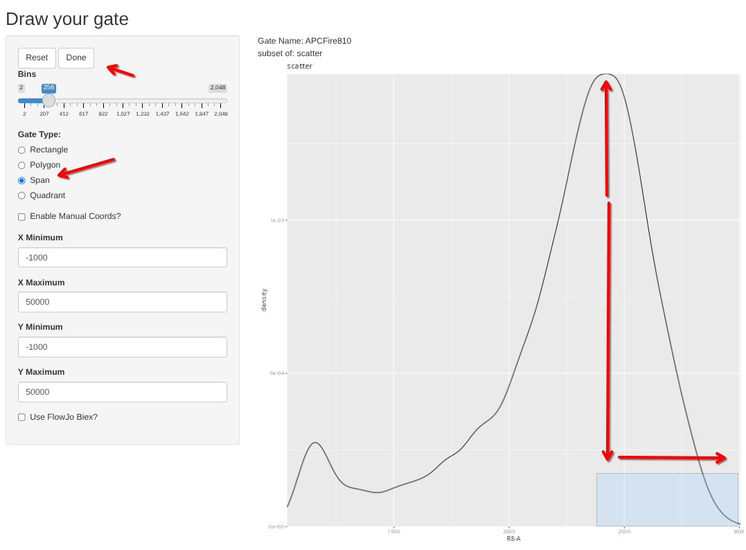
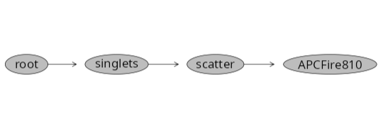
.
And remember, if we need to adjust the gate after the fact, we can do so via the new gs_gate_interative_adjust() function.
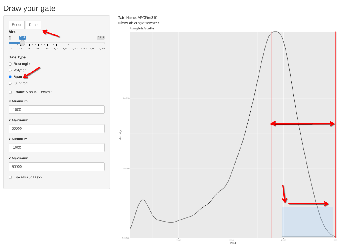
.
We will also need an internal “negative” gate for a couple examples, so lets draw its own span gate.
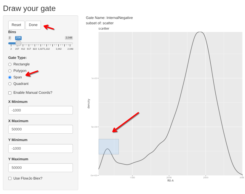
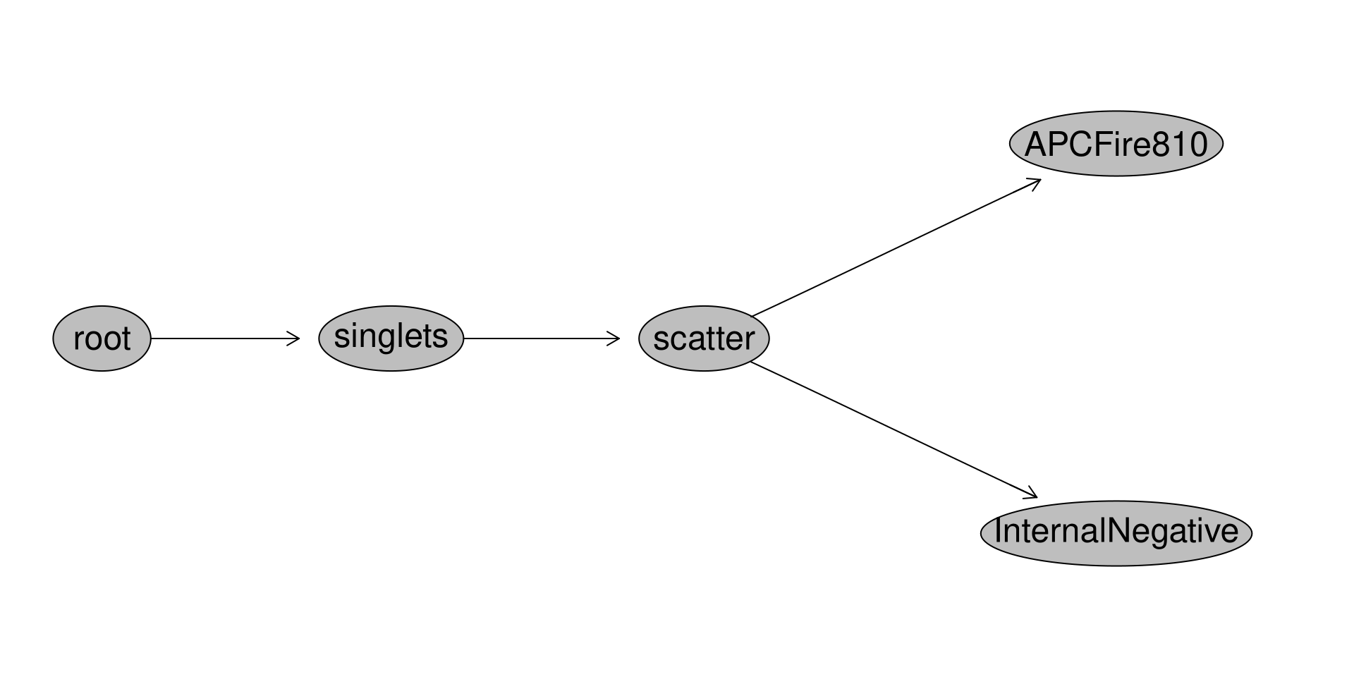
Extracting Exprs
.
With our span gates created, we are now at the point that we can extract the exprs matrices. To do this, we first need to retrieve from the GatingSet a cytoset corresponding to just our gated cells (via the gs_pop_get_data() function). Remember, this is the step where we need to specify the “inverse.transform=TRUE” argument, so that we reverse the applied transformation from earlier.
.
At this point, we can use the exprs() helper function to retrieve the underlying data being stored under the “exprs” slot. We can also make our lives simpler by converting from a matrix over to a data.frame, enabling use of the dplyr package functions for several of the subsequent steps.
    Time    UV1-A    UV2-A     UV3-A     UV4-A    UV5-A    UV6-A    UV7-A
1 521939 641.7078 589.1987 1074.3470 1058.2816 1032.845 1901.992 4073.742
2  18412 153.5099 139.0814  691.3152  402.6661 1014.623 1298.513 2765.412
3 164186 116.5459 720.0988  269.3858  567.9276 1149.465 1488.170 3432.184
     UV8-A    UV9-A   UV10-A    UV11-A    UV12-A    UV13-A    UV14-A    UV15-A
1 2631.536 2337.457 991.6415 3273.9131 2324.6646 1510.7793 1719.4755 2032.8173
2 2353.597 2220.689 996.1790 2417.4846 1383.9696 1036.8619 1292.1914 1789.8342
3 2119.241 1511.151 761.6002  817.3074  991.9396  180.2108  497.0484  759.1456
    UV16-A    SSC-W   SSC-H   SSC-A     V1-A     V2-A     V3-A     V4-A
1 7380.604 670261.9 1023604 1143471 851.1250 3566.819 4903.525 5478.481
2 5465.298 687311.4 1050826 1203741 427.4191 1557.737 2713.356 3466.100
3 3629.500 639144.4 1002897 1068327 448.1815 2087.387 3081.719 3676.131
      V5-A     V6-A     V7-A     V8-A     V9-A    V10-A     V11-A    V12-A
1 7382.444 6454.525 8553.464 6269.176 4711.025 5532.175 11721.944 5689.200
2 4781.082 5320.149 6556.961 5045.149 4408.387 5030.369  7062.138 3361.256
3 4396.150 4661.457 6704.844 4425.645 3920.676 4792.631  4639.732 2316.875
     V13-A    V14-A    V15-A    V16-A    FSC-W   FSC-H   FSC-A  SSC-B-W SSC-B-H
1 4920.988 4275.219 7053.544 13972.89 674506.7 1420303 1596673 665733.4  741211
2 3707.756 2138.262 5415.506 12034.34 680553.9 1493093 1693550 693400.6  637423
3 2186.800 2023.725 3330.937  7345.87 678422.8 1482793 1676601 645656.9  626490
   SSC-B-A     B1-A     B2-A     B3-A     B4-A     B5-A     B6-A     B7-A
1 822414.9 2065.505 2742.674 3271.125 2088.320 2132.650 1895.595 2972.970
2 736649.1 1282.970 1882.204 3345.940 2587.649 2044.575 1692.730 2815.670
3 674162.6 1932.255 3140.995 3238.755 2450.369 2592.720 2072.915 1902.615
      B8-A     B9-A     B10-A    B11-A    B12-A      B13-A    B14-A     YG1-A
1 1628.640 2463.174 1184.1703 918.8395 760.2395  917.02032 3089.775 1018.4301
2 1691.495 1615.250  935.7395 386.1001 729.0402   24.50534 3250.065  962.8499
3 1553.955 1214.005  360.4247 622.7646 271.7649 1434.42004 2259.660 1048.8799
    YG2-A   YG3-A     YG4-A     YG5-A    YG6-A     YG7-A    YG8-A    YG9-A
1 1080.17 2121.07 20503.355 13645.522 10438.40 13630.612 5722.570 7794.431
2 1844.15 1819.16 13175.257  8777.441  6281.17  8347.921 4560.641 6547.939
3 1079.89 2188.34  5942.581  4584.930  2754.92  4348.470 1776.810 3512.740
    YG10-A     R1-A      R2-A      R3-A     R4-A     R5-A      R6-A     R7-A
1 20962.00 37950.85 37463.023 28257.102 22815.74 20428.87 14737.938 32214.97
2 18233.39 24004.75 23490.387 19048.469 15905.61 13671.14  9155.021 25338.94
3 11093.81  9807.70  9904.511  8169.281  6269.90  5548.97  4252.011 14647.71
      R8-A
1 70631.25
2 61678.40
3 37278.79
.
Before moving too far ahead, having been burned by transforms that failed to untransform in the past, lets double check to make sure these retrieved values look “raw” and are not still biexponentially-transformed.
      Time            UV1-A            UV2-A            UV3-A
 Min.   :    84   Min.   :-833.6   Min.   :-567.0   Min.   :-617.2
 1st Qu.:147481   1st Qu.: 104.6   1st Qu.: 408.1   1st Qu.: 368.1
 Median :287356   Median : 333.1   Median : 646.6   Median : 590.6
 Mean   :293512   Mean   : 340.4   Mean   : 652.3   Mean   : 586.0
 3rd Qu.:440190   3rd Qu.: 578.3   3rd Qu.: 887.4   3rd Qu.: 799.9
 Max.   :603617   Max.   :1736.8   Max.   :1918.7   Max.   :1710.0
     UV4-A            UV5-A            UV6-A            UV7-A
 Min.   :-321.8   Min.   :-101.4   Min.   : 203.6   Min.   :1122
 1st Qu.: 473.6   1st Qu.: 781.5   1st Qu.:1334.8   1st Qu.:2736
 Median : 704.6   Median :1008.2   Median :1652.0   Median :3248
 Mean   : 706.6   Mean   :1017.8   Mean   :1646.6   Mean   :3246
 3rd Qu.: 934.4   3rd Qu.:1254.2   3rd Qu.:1959.7   3rd Qu.:3751
 Max.   :2079.1   Max.   :2506.0   Max.   :3298.2   Max.   :5869
     UV8-A            UV9-A            UV10-A           UV11-A
 Min.   : 513.8   Min.   : 532.4   Min.   :-484.1   Min.   : 198.9
 1st Qu.:2038.2   1st Qu.:1847.0   1st Qu.: 728.9   1st Qu.:1486.6
 Median :2400.8   Median :2243.9   Median : 973.0   Median :1891.1
 Mean   :2403.1   Mean   :2253.3   Mean   : 973.4   Mean   :2009.3
 3rd Qu.:2770.1   3rd Qu.:2632.4   3rd Qu.:1217.9   3rd Qu.:2394.7
 Max.   :4434.2   Max.   :5861.9   Max.   :2167.7   Max.   :8012.7
     UV12-A           UV13-A           UV14-A           UV15-A
 Min.   :-392.0   Min.   :-385.5   Min.   :-334.7   Min.   :-228.7
 1st Qu.: 723.2   1st Qu.: 620.8   1st Qu.: 731.5   1st Qu.:1001.3
 Median : 996.2   Median : 867.0   Median :1011.8   Median :1303.1
 Mean   :1029.5   Mean   : 911.9   Mean   :1051.4   Mean   :1368.6
 3rd Qu.:1290.1   3rd Qu.:1167.7   3rd Qu.:1338.4   3rd Qu.:1651.5
 Max.   :3484.7   Max.   :3073.7   Max.   :4076.9   Max.   :4091.9
     UV16-A          SSC-W             SSC-H             SSC-A
 Min.   : 1597   Min.   : 607182   Min.   : 449888   Min.   : 511812
 1st Qu.: 3165   1st Qu.: 661148   1st Qu.: 806612   1st Qu.: 913448
 Median : 3816   Median : 675745   Median : 937618   Median :1065911
 Mean   : 4193   Mean   : 683548   Mean   : 939551   Mean   :1069927
 3rd Qu.: 4849   3rd Qu.: 692358   3rd Qu.:1063775   3rd Qu.:1218457
 Max.   :13678   Max.   :1208521   Max.   :1483718   Max.   :1667566
      V1-A             V2-A             V3-A           V4-A
 Min.   :-366.5   Min.   : 623.4   Min.   :1274   Min.   :1257
 1st Qu.: 406.0   1st Qu.:1761.4   1st Qu.:2929   1st Qu.:3313
 Median : 621.3   Median :2145.9   Median :3540   Median :3979
 Mean   : 619.3   Mean   :2155.6   Mean   :3585   Mean   :4027
 3rd Qu.: 821.8   3rd Qu.:2533.5   3rd Qu.:4165   3rd Qu.:4697
 Max.   :1764.0   Max.   :5111.1   Max.   :8373   Max.   :8846
      V5-A            V6-A            V7-A            V8-A            V9-A
 Min.   : 2003   Min.   : 2057   Min.   : 2957   Min.   : 2386   Min.   :1562
 1st Qu.: 4871   1st Qu.: 4649   1st Qu.: 6421   1st Qu.: 4882   1st Qu.:3457
 Median : 5779   Median : 5472   Median : 7569   Median : 5764   Median :4092
 Mean   : 5813   Mean   : 5475   Mean   : 7566   Mean   : 5732   Mean   :4071
 3rd Qu.: 6688   3rd Qu.: 6290   3rd Qu.: 8660   3rd Qu.: 6562   3rd Qu.:4670
 Max.   :11845   Max.   :10657   Max.   :14347   Max.   :10441   Max.   :7723
     V10-A          V11-A           V12-A             V13-A
 Min.   :1890   Min.   : 1481   Min.   :  842.3   Min.   :  617.2
 1st Qu.:4084   1st Qu.: 4951   1st Qu.: 2449.2   1st Qu.: 2291.8
 Median :4803   Median : 6108   Median : 3003.4   Median : 2829.7
 Mean   :4795   Mean   : 6532   Mean   : 3167.8   Mean   : 2993.3
 3rd Qu.:5495   3rd Qu.: 7604   3rd Qu.: 3692.5   3rd Qu.: 3503.9
 Max.   :8674   Max.   :24117   Max.   :10455.5   Max.   :10972.6
     V14-A            V15-A           V16-A           FSC-W
 Min.   : 340.2   Min.   : 1661   Min.   : 4379   Min.   :635088
 1st Qu.:1953.9   1st Qu.: 3058   1st Qu.: 6395   1st Qu.:666236
 Median :2422.5   Median : 3647   Median : 7657   Median :672919
 Mean   :2551.4   Mean   : 3916   Mean   : 8550   Mean   :674482
 3rd Qu.:3001.8   3rd Qu.: 4524   3rd Qu.: 9844   3rd Qu.:680558
 Max.   :8687.0   Max.   :11154   Max.   :25874   Max.   :741803
     FSC-H             FSC-A            SSC-B-W           SSC-B-H
 Min.   : 999096   Min.   :1180213   Min.   : 618274   Min.   : 293280
 1st Qu.:1311526   1st Qu.:1467756   1st Qu.: 657644   1st Qu.: 566948
 Median :1400595   Median :1572188   Median : 670419   Median : 653508
 Mean   :1396976   Mean   :1570965   Mean   : 677396   Mean   : 661754
 3rd Qu.:1486583   3rd Qu.:1674545   3rd Qu.: 684631   3rd Qu.: 754072
 Max.   :1692027   Max.   :1940438   Max.   :1194018   Max.   :1138188
    SSC-B-A             B1-A             B2-A             B3-A
 Min.   : 316600   Min.   : 545.5   Min.   : 783.3   Min.   :1057
 1st Qu.: 636121   1st Qu.:1527.8   1st Qu.:2002.3   1st Qu.:2973
 Median : 737487   Median :1827.9   Median :2365.2   Median :3449
 Mean   : 746907   Mean   :1843.6   Mean   :2370.3   Mean   :3467
 3rd Qu.: 854497   3rd Qu.:2137.5   3rd Qu.:2718.8   3rd Qu.:3926
 Max.   :1316862   Max.   :3928.7   Max.   :4949.4   Max.   :6545
      B4-A             B5-A             B6-A             B7-A
 Min.   : 727.3   Min.   : 601.6   Min.   : 239.1   Min.   : 338.7
 1st Qu.:2151.0   1st Qu.:1912.4   1st Qu.:1584.0   1st Qu.:1657.8
 Median :2530.7   Median :2277.0   Median :1892.1   Median :2047.5
 Mean   :2541.5   Mean   :2276.9   Mean   :1892.6   Mean   :2108.8
 3rd Qu.:2920.1   3rd Qu.:2622.5   3rd Qu.:2184.5   3rd Qu.:2475.3
 Max.   :4651.1   Max.   :4556.9   Max.   :3560.6   Max.   :5871.2
      B8-A             B9-A             B10-A            B11-A
 Min.   : 172.5   Min.   :  63.18   Min.   :-161.8   Min.   :-274.0
 1st Qu.:1183.6   1st Qu.:1146.41   1st Qu.: 685.3   1st Qu.: 465.1
 Median :1471.1   Median :1420.97   Median : 913.0   Median : 698.6
 Mean   :1505.0   Mean   :1459.30   Mean   : 928.2   Mean   : 708.8
 3rd Qu.:1787.2   3rd Qu.:1738.55   3rd Qu.:1155.2   3rd Qu.: 939.6
 Max.   :4220.0   Max.   :3784.95   Max.   :2875.4   Max.   :2164.3
     B12-A            B13-A            B14-A            YG1-A
 Min.   :-448.4   Min.   :-340.1   Min.   : 774.3   Min.   :  40.53
 1st Qu.: 426.1   1st Qu.: 496.8   1st Qu.:1739.8   1st Qu.:1071.38
 Median : 629.3   Median : 717.3   Median :2117.2   Median :1325.17
 Mean   : 637.5   Mean   : 732.3   Mean   :2287.8   Mean   :1329.64
 3rd Qu.: 837.3   3rd Qu.: 948.1   3rd Qu.:2675.3   3rd Qu.:1582.91
 Max.   :2143.3   Max.   :2135.6   Max.   :6776.4   Max.   :2705.71
     YG2-A            YG3-A             YG4-A           YG5-A
 Min.   : -61.6   Min.   :  16.52   Min.   : 2185   Min.   :  889.1
 1st Qu.:1134.1   1st Qu.:1603.77   1st Qu.: 7341   1st Qu.: 5064.0
 Median :1425.2   Median :1951.60   Median : 9419   Median : 6529.7
 Mean   :1420.7   Mean   :1941.97   Mean   :10520   Mean   : 7229.9
 3rd Qu.:1694.4   3rd Qu.:2278.95   3rd Qu.:12558   3rd Qu.: 8669.1
 Max.   :2756.8   Max.   :3900.68   Max.   :49143   Max.   :33692.5
     YG6-A           YG7-A           YG8-A             YG9-A
 Min.   : 1019   Min.   : 1422   Min.   :  522.4   Min.   : 1654
 1st Qu.: 3692   1st Qu.: 4932   1st Qu.: 2310.0   1st Qu.: 3476
 Median : 4643   Median : 6287   Median : 3031.4   Median : 4221
 Mean   : 5082   Mean   : 6945   Mean   : 3318.8   Mean   : 4621
 3rd Qu.: 6028   3rd Qu.: 8261   3rd Qu.: 4006.6   3rd Qu.: 5358
 Max.   :21549   Max.   :30490   Max.   :15270.9   Max.   :15624
     YG10-A           R1-A            R2-A            R3-A
 Min.   : 6912   Min.   : 3122   Min.   : 2823   Min.   : 2585
 1st Qu.: 9577   1st Qu.:12751   1st Qu.:12207   1st Qu.:10000
 Median :11512   Median :16804   Median :16106   Median :13048
 Mean   :12887   Mean   :18972   Mean   :18115   Mean   :14516
 3rd Qu.:14823   3rd Qu.:22957   3rd Qu.:21920   3rd Qu.:17441
 Max.   :40375   Max.   :93836   Max.   :88220   Max.   :65785
      R4-A            R5-A            R6-A            R7-A
 Min.   : 2245   Min.   : 1695   Min.   : 1868   Min.   : 9676
 1st Qu.: 8243   1st Qu.: 6896   1st Qu.: 5175   1st Qu.:13876
 Median :10710   Median : 9062   Median : 6715   Median :16692
 Mean   :11963   Mean   :10163   Mean   : 7506   Mean   :18598
 3rd Qu.:14353   3rd Qu.:12275   3rd Qu.: 9011   3rd Qu.:21545
 Max.   :54530   Max.   :49047   Max.   :35646   Max.   :60396
      R8-A
 Min.   : 26680
 1st Qu.: 31867
 Median : 38226
 Mean   : 43115
 3rd Qu.: 49828
 Max.   :137221
.
So far so good! (since I am seeing negative values on lower end, ranging up through biexponential, all varying by fluorophore). We can then proceed and repeat the process of extracting out the underlying data for our internal negative as well.
    Time     UV1-A    UV2-A     UV3-A      UV4-A     UV5-A    UV6-A    UV7-A
1  37476 574.69519 721.9586  761.0048  820.43085 1209.1887 1728.624 3326.348
2 179720  67.90479 562.3496  232.1990 1347.89868 1019.5323 1815.642 2997.387
3 378517 216.28224 279.7248 1199.9666  -74.44981  800.9441 1503.639 3320.100
     UV8-A    UV9-A   UV10-A   UV11-A   UV12-A   UV13-A   UV14-A    UV15-A
1 2116.043 2448.722 621.0314 646.9134 205.5729 133.9492 525.7569  454.4310
2 1916.421 2149.511 916.3739 765.4676 707.6783 403.1870 618.1310  347.4803
3 2662.997 2372.414 621.7749 659.5576 257.1888 558.3334 361.4630 -177.8309
    UV16-A    SSC-W   SSC-H     SSC-A     V1-A     V2-A     V3-A     V4-A
1 262.9158 660806.4 1016762 1119804.9 948.0623 2050.882 4383.913 4227.781
2 152.8411 653952.9  560464  610861.8 649.8937 1573.413 2951.643 3583.800
3 169.9469 704944.6  799284  939084.8 386.0315 2380.675 3552.518 3858.869
      V5-A     V6-A     V7-A     V8-A     V9-A    V10-A    V11-A    V12-A
1 5319.738 4942.025 7542.495 5047.007 4334.894 4705.388 2797.781 1410.338
2 5462.600 5052.575 7003.700 5157.969 3729.619 3827.519 2675.957 1048.850
3 5861.213 5718.350 7996.657 5301.725 4099.494 5365.250 2539.694 1778.150
     V13-A     V14-A     V15-A    V16-A    FSC-W   FSC-H   FSC-A  SSC-B-W
1 1426.356 1067.2067 1466.0936 881.7188 678730.9 1377827 1558623 663281.9
2 1113.956 1035.7190 1368.9503 661.9940 664194.0 1435669 1589271 657571.0
3 1532.231  939.8808  787.4626 692.7251 686260.4 1353584 1548185 699355.2
  SSC-B-H  SSC-B-A     B1-A     B2-A     B3-A    B4-A     B5-A     B6-A
1  650077 718640.5 2165.735 2539.939 3688.359 3060.98 2613.195 1603.680
2  409499 448791.1 1949.934 2010.710 2940.925 1568.32 1407.900 1712.685
3  541047 630640.1 1858.610 2324.985 3700.645 2577.38 2713.360 1640.339
       B7-A      B8-A      B9-A    B10-A    B11-A    B12-A    B13-A    B14-A
1 1393.0800  700.9597 1223.7551 468.4551 787.9304 675.3495 197.5996 694.1999
2  680.0302 1053.2601  650.5199 566.7355 415.8705 802.4898 916.1755 422.2401
3 1210.1050  734.5649 1476.5399 773.2403 518.1148 297.6996 382.9148 131.0398
    YG1-A     YG2-A   YG3-A   YG4-A   YG5-A     YG6-A     YG7-A      YG8-A
1 1551.55  702.1004 1218.84 1926.47 1193.01  562.5896 1271.8303 1011.78046
2 1344.70 1209.1100 1456.28 2230.48 1237.25  301.2104 1282.6095  748.22968
3 1349.39 1552.6000 2437.26 1198.05 1780.59 1399.0895  827.1895   51.17008
     YG9-A   YG10-A      R1-A      R2-A      R3-A      R4-A      R5-A     R6-A
1 158.0599 245.9796 1274.7698 1422.7500 1272.5996 1373.3997  743.1900 577.5001
2 817.0403 401.1701  835.0997 1516.8995  719.4598  739.8304  265.9998 829.2202
3 745.9195 491.0496  514.7100  827.3996  952.5599  266.1398 1005.4102 540.1902
      R7-A    R8-A
1 569.1695 1079.68
2 553.7001 1316.70
3 610.7504 1282.12 Time UV1-A UV2-A UV3-A
Min. : 603 Min. :-781.3 Min. :-530.3 Min. :-287.2
1st Qu.:168610 1st Qu.: 109.6 1st Qu.: 375.9 1st Qu.: 359.3
Median :305856 Median : 310.3 Median : 635.1 Median : 591.9
Mean :305453 Mean : 327.7 Mean : 633.5 Mean : 591.3
3rd Qu.:457748 3rd Qu.: 537.7 3rd Qu.: 887.6 3rd Qu.: 807.4
Max. :601230 Max. :1299.7 Max. :2197.8 Max. :1782.3
UV4-A UV5-A UV6-A UV7-A
Min. :-229.4 Min. :-165.9 Min. : 364.5 Min. :1088
1st Qu.: 471.7 1st Qu.: 742.0 1st Qu.:1304.4 1st Qu.:2617
Median : 663.2 Median : 979.1 Median :1567.9 Median :3053
Mean : 693.2 Mean :1005.1 Mean :1601.4 Mean :3125
3rd Qu.: 918.6 3rd Qu.:1229.5 3rd Qu.:1827.0 3rd Qu.:3471
Max. :2375.4 Max. :2690.6 Max. :5144.8 Max. :9015
UV8-A UV9-A UV10-A UV11-A
Min. : 740 Min. : 617.8 Min. :-142.0 Min. :-160.7
1st Qu.:1960 1st Qu.:1801.5 1st Qu.: 647.1 1st Qu.: 462.1
Median :2270 Median :2145.6 Median : 929.6 Median : 662.0
Mean :2323 Mean :2178.3 Mean : 920.8 Mean : 682.0
3rd Qu.:2633 3rd Qu.:2512.2 3rd Qu.:1164.6 3rd Qu.: 889.2
Max. :6432 Max. :6036.7 Max. :2548.9 Max. :1849.3
UV12-A UV13-A UV14-A UV15-A
Min. :-405.7 Min. :-484.2 Min. :-470.0 Min. :-571.8
1st Qu.: 252.3 1st Qu.: 130.0 1st Qu.: 184.3 1st Qu.: 120.2
Median : 437.5 Median : 329.0 Median : 408.4 Median : 307.4
Mean : 434.0 Mean : 320.2 Mean : 415.9 Mean : 318.2
3rd Qu.: 625.8 3rd Qu.: 508.5 3rd Qu.: 621.3 3rd Qu.: 517.7
Max. :1397.7 Max. :1351.4 Max. :1731.7 Max. :1438.1
UV16-A SSC-W SSC-H SSC-A
Min. :-750.82 Min. : 626198 Min. : 471628 Min. : 537994
1st Qu.: 71.29 1st Qu.: 661212 1st Qu.: 749651 1st Qu.: 850046
Median : 318.96 Median : 677648 Median : 857858 Median : 981290
Mean : 310.00 Mean : 696004 Mean : 870984 Mean :1009417
3rd Qu.: 542.12 3rd Qu.: 709054 3rd Qu.: 991487 3rd Qu.:1153504
Max. :1137.49 Max. :1096566 Max. :1427156 Max. :1660615
V1-A V2-A V3-A V4-A
Min. :-397.6 Min. : 751.4 Min. : 1447 Min. : 1741
1st Qu.: 418.1 1st Qu.: 1722.1 1st Qu.: 2894 1st Qu.: 3223
Median : 606.4 Median : 2059.6 Median : 3349 Median : 3776
Mean : 617.4 Mean : 2157.0 Mean : 3522 Mean : 3961
3rd Qu.: 802.7 3rd Qu.: 2432.4 3rd Qu.: 3839 3rd Qu.: 4270
Max. :2756.8 Max. :10084.7 Max. :18392 Max. :19601
V5-A V6-A V7-A V8-A
Min. : 2536 Min. : 2717 Min. : 4004 Min. : 2963
1st Qu.: 4723 1st Qu.: 4509 1st Qu.: 6275 1st Qu.: 4821
Median : 5547 Median : 5210 Median : 7238 Median : 5522
Mean : 5717 Mean : 5373 Mean : 7437 Mean : 5681
3rd Qu.: 6240 3rd Qu.: 5847 3rd Qu.: 8047 3rd Qu.: 6178
Max. :24513 Max. :20324 Max. :24204 Max. :17562
V9-A V10-A V11-A V12-A V13-A
Min. : 2073 Min. : 2315 Min. :1067 Min. : 442.3 Min. : 266
1st Qu.: 3403 1st Qu.: 3922 1st Qu.:2233 1st Qu.:1210.4 1st Qu.:1099
Median : 3894 Median : 4475 Median :2576 Median :1465.2 Median :1332
Mean : 3988 Mean : 4608 Mean :2639 Mean :1487.7 Mean :1360
3rd Qu.: 4396 3rd Qu.: 5099 3rd Qu.:2966 3rd Qu.:1728.8 3rd Qu.:1593
Max. :12572 Max. :13652 Max. :7500 Max. :4285.9 Max. :3904
V14-A V15-A V16-A FSC-W
Min. : 265.0 Min. :-171.1 Min. :-232.3 Min. :641243
1st Qu.: 900.8 1st Qu.: 775.1 1st Qu.: 419.8 1st Qu.:666225
Median :1166.8 Median :1005.6 Median : 622.4 Median :673760
Mean :1180.2 Mean :1021.5 Mean : 631.4 Mean :678202
3rd Qu.:1433.3 3rd Qu.:1269.5 3rd Qu.: 851.7 3rd Qu.:685076
Max. :3547.8 Max. :2293.4 Max. :1616.4 Max. :771190
FSC-H FSC-A SSC-B-W SSC-B-H
Min. : 925729 Min. :1183497 Min. : 628308 Min. : 338898
1st Qu.:1248164 1st Qu.:1412138 1st Qu.: 657497 1st Qu.: 507502
Median :1352210 Median :1520434 Median : 671368 Median : 587826
Mean :1338199 Mean :1511225 Mean : 688859 Mean : 599989
3rd Qu.:1437331 3rd Qu.:1616516 3rd Qu.: 700817 3rd Qu.: 677992
Max. :1652109 Max. :1897885 Max. :1119866 Max. :1149877
SSC-B-A B1-A B2-A B3-A
Min. : 385982 Min. : 579.3 Min. :1007 Min. : 1752
1st Qu.: 582052 1st Qu.:1543.4 1st Qu.:2030 1st Qu.: 2957
Median : 671807 Median :1831.9 Median :2339 Median : 3405
Mean : 687380 Mean :1887.8 Mean :2421 Mean : 3514
3rd Qu.: 780042 3rd Qu.:2158.2 3rd Qu.:2755 3rd Qu.: 3975
Max. :1268330 Max. :6094.9 Max. :7776 Max. :10097
B4-A B5-A B6-A B7-A
Min. :1080 Min. : 819.3 Min. : 409.4 Min. : 353.1
1st Qu.:2103 1st Qu.:1879.8 1st Qu.:1557.4 1st Qu.:1130.1
Median :2471 Median :2230.8 Median :1847.6 Median :1358.8
Mean :2540 Mean :2269.8 Mean :1875.6 Mean :1388.0
3rd Qu.:2915 3rd Qu.:2591.4 3rd Qu.:2135.2 3rd Qu.:1597.1
Max. :7882 Max. :6503.3 Max. :5278.6 Max. :3794.2
B8-A B9-A B10-A B11-A
Min. : 134.4 Min. : 24.57 Min. :-247.1 Min. :-390.8
1st Qu.: 803.6 1st Qu.: 830.39 1st Qu.: 450.7 1st Qu.: 288.4
Median :1024.8 Median :1045.69 Median : 641.7 Median : 484.4
Mean :1028.9 Mean :1068.73 Mean : 648.6 Mean : 477.5
3rd Qu.:1260.6 3rd Qu.:1286.28 3rd Qu.: 838.0 3rd Qu.: 673.2
Max. :3140.9 Max. :3372.85 Max. :1821.6 Max. :1400.2
B12-A B13-A B14-A YG1-A
Min. :-267.7 Min. :-444.7 Min. :-413.5 Min. : 325.9
1st Qu.: 240.2 1st Qu.: 176.0 1st Qu.: 209.2 1st Qu.: 987.6
Median : 433.5 Median : 347.6 Median : 403.8 Median :1219.2
Mean : 442.3 Mean : 353.1 Mean : 412.6 Mean :1231.9
3rd Qu.: 624.3 3rd Qu.: 526.7 3rd Qu.: 601.2 3rd Qu.:1470.2
Max. :1857.9 Max. :1269.9 Max. :1539.7 Max. :2779.1
YG2-A YG3-A YG4-A YG5-A
Min. :-215.1 Min. : 284 Min. : 355.6 Min. : 47.95
1st Qu.:1061.4 1st Qu.:1279 1st Qu.:1248.2 1st Qu.: 886.67
Median :1310.2 Median :1588 Median :1568.5 Median :1144.43
Mean :1311.2 Mean :1610 Mean :1607.6 Mean :1156.88
3rd Qu.:1550.0 3rd Qu.:1925 3rd Qu.:1925.5 3rd Qu.:1389.13
Max. :3508.2 Max. :3464 Max. :4352.9 Max. :2977.66
YG6-A YG7-A YG8-A YG9-A
Min. :-189.2 Min. : -94.22 Min. :-641.6 Min. :-388.5
1st Qu.: 755.1 1st Qu.: 945.23 1st Qu.: 324.9 1st Qu.: 268.3
Median :1033.4 Median :1246.42 Median : 543.8 Median : 498.7
Mean :1051.0 Mean :1265.33 Mean : 553.9 Mean : 512.2
3rd Qu.:1338.4 3rd Qu.:1543.22 3rd Qu.: 796.1 3rd Qu.: 724.5
Max. :2414.5 Max. :3045.42 Max. :1477.4 Max. :1696.4
YG10-A R1-A R2-A R3-A
Min. :-451.4 Min. :-262.8 Min. :-216.3 Min. :-126.9
1st Qu.: 173.7 1st Qu.: 435.0 1st Qu.: 522.8 1st Qu.: 463.9
Median : 401.1 Median : 640.1 Median : 754.1 Median : 715.2
Mean : 408.6 Mean : 733.9 Mean : 811.9 Mean : 756.8
3rd Qu.: 617.9 3rd Qu.: 958.0 3rd Qu.:1020.4 3rd Qu.: 993.4
Max. :1347.8 Max. :4036.6 Max. :3765.6 Max. :3043.0
R4-A R5-A R6-A R7-A
Min. :-189.5 Min. :-550.9 Min. :-466.3 Min. :-561.3
1st Qu.: 441.5 1st Qu.: 280.0 1st Qu.: 151.9 1st Qu.: 200.4
Median : 680.2 Median : 520.1 Median : 348.8 Median : 494.5
Mean : 702.2 Mean : 512.1 Mean : 373.2 Mean : 498.2
3rd Qu.: 926.3 3rd Qu.: 740.1 3rd Qu.: 581.1 3rd Qu.: 748.1
Max. :2338.1 Max. :2264.7 Max. :1681.0 Max. :2032.2
R8-A
Min. :-425.6
1st Qu.: 271.5
Median : 600.0
Mean : 645.8
3rd Qu.: 984.3
Max. :1798.5 .
Glancing at the summary() data for our InternalNegative, we can see that the R8 detector is definitely lower than where we expect to see the autofluorescence peaks (typically UV7, V7 or B3), so for this particular control it doesn’t look like we are dealing with non-specific staining substantially affecting our internal negative cells. This is not always the case for individual fluorophores, so it is worth checking.
Removing FSC SSC Time
.
Before we can get to the fluorescent signature itself, we first need to remove from our data.frames the columns that do not correspond to fluorescent detectors. In this case, these will be the FSC, SSC and Time columns (and their -A, -H and -W variants).
 [1] "Time"    "UV1-A"   "UV2-A"   "UV3-A"   "UV4-A"   "UV5-A"   "UV6-A"
 [8] "UV7-A"   "UV8-A"   "UV9-A"   "UV10-A"  "UV11-A"  "UV12-A"  "UV13-A"
[15] "UV14-A"  "UV15-A"  "UV16-A"  "SSC-W"   "SSC-H"   "SSC-A"   "V1-A"
[22] "V2-A"    "V3-A"    "V4-A"    "V5-A"    "V6-A"    "V7-A"    "V8-A"
[29] "V9-A"    "V10-A"   "V11-A"   "V12-A"   "V13-A"   "V14-A"   "V15-A"
[36] "V16-A"   "FSC-W"   "FSC-H"   "FSC-A"   "SSC-B-W" "SSC-B-H" "SSC-B-A"
[43] "B1-A"    "B2-A"    "B3-A"    "B4-A"    "B5-A"    "B6-A"    "B7-A"
[50] "B8-A"    "B9-A"    "B10-A"   "B11-A"   "B12-A"   "B13-A"   "B14-A"
[57] "YG1-A"   "YG2-A"   "YG3-A"   "YG4-A"   "YG5-A"   "YG6-A"   "YG7-A"
[64] "YG8-A"   "YG9-A"   "YG10-A"  "R1-A"    "R2-A"    "R3-A"    "R4-A"
[71] "R5-A"    "R6-A"    "R7-A"    "R8-A"
.
We can repurpose the code we used at the transformation step (alongside use of stringr str_detect()) to select for columns that don’t match the character strings that contain “FSC”, “SSC” or “Time”, which will leave us with just the fluorescent detectors
     UV1-A    UV2-A     UV3-A     UV4-A    UV5-A    UV6-A    UV7-A    UV8-A
1 641.7078 589.1987 1074.3470 1058.2816 1032.845 1901.992 4073.742 2631.536
2 153.5099 139.0814  691.3152  402.6661 1014.623 1298.513 2765.412 2353.597
3 116.5459 720.0988  269.3858  567.9276 1149.465 1488.170 3432.184 2119.241
     UV9-A   UV10-A    UV11-A    UV12-A    UV13-A    UV14-A    UV15-A   UV16-A
1 2337.457 991.6415 3273.9131 2324.6646 1510.7793 1719.4755 2032.8173 7380.604
2 2220.689 996.1790 2417.4846 1383.9696 1036.8619 1292.1914 1789.8342 5465.298
3 1511.151 761.6002  817.3074  991.9396  180.2108  497.0484  759.1456 3629.500
      V1-A     V2-A     V3-A     V4-A     V5-A     V6-A     V7-A     V8-A
1 851.1250 3566.819 4903.525 5478.481 7382.444 6454.525 8553.464 6269.176
2 427.4191 1557.737 2713.356 3466.100 4781.082 5320.149 6556.961 5045.149
3 448.1815 2087.387 3081.719 3676.131 4396.150 4661.457 6704.844 4425.645
      V9-A    V10-A     V11-A    V12-A    V13-A    V14-A    V15-A    V16-A
1 4711.025 5532.175 11721.944 5689.200 4920.988 4275.219 7053.544 13972.89
2 4408.387 5030.369  7062.138 3361.256 3707.756 2138.262 5415.506 12034.34
3 3920.676 4792.631  4639.732 2316.875 2186.800 2023.725 3330.937  7345.87
      B1-A     B2-A     B3-A     B4-A     B5-A     B6-A     B7-A     B8-A
1 2065.505 2742.674 3271.125 2088.320 2132.650 1895.595 2972.970 1628.640
2 1282.970 1882.204 3345.940 2587.649 2044.575 1692.730 2815.670 1691.495
3 1932.255 3140.995 3238.755 2450.369 2592.720 2072.915 1902.615 1553.955
      B9-A     B10-A    B11-A    B12-A      B13-A    B14-A     YG1-A   YG2-A
1 2463.174 1184.1703 918.8395 760.2395  917.02032 3089.775 1018.4301 1080.17
2 1615.250  935.7395 386.1001 729.0402   24.50534 3250.065  962.8499 1844.15
3 1214.005  360.4247 622.7646 271.7649 1434.42004 2259.660 1048.8799 1079.89
    YG3-A     YG4-A     YG5-A    YG6-A     YG7-A    YG8-A    YG9-A   YG10-A
1 2121.07 20503.355 13645.522 10438.40 13630.612 5722.570 7794.431 20962.00
2 1819.16 13175.257  8777.441  6281.17  8347.921 4560.641 6547.939 18233.39
3 2188.34  5942.581  4584.930  2754.92  4348.470 1776.810 3512.740 11093.81
      R1-A      R2-A      R3-A     R4-A     R5-A      R6-A     R7-A     R8-A
1 37950.85 37463.023 28257.102 22815.74 20428.87 14737.938 32214.97 70631.25
2 24004.75 23490.387 19048.469 15905.61 13671.14  9155.021 25338.94 61678.40
3  9807.70  9904.511  8169.281  6269.90  5548.97  4252.011 14647.71 37278.79
.
We can then repeat this process for our negative background data, so that both data.frame objects are comparable to each other.
      UV1-A    UV2-A     UV3-A      UV4-A     UV5-A    UV6-A    UV7-A    UV8-A
1 574.69519 721.9586  761.0048  820.43085 1209.1887 1728.624 3326.348 2116.043
2  67.90479 562.3496  232.1990 1347.89868 1019.5323 1815.642 2997.387 1916.421
3 216.28224 279.7248 1199.9666  -74.44981  800.9441 1503.639 3320.100 2662.997
     UV9-A   UV10-A   UV11-A   UV12-A   UV13-A   UV14-A    UV15-A   UV16-A
1 2448.722 621.0314 646.9134 205.5729 133.9492 525.7569  454.4310 262.9158
2 2149.511 916.3739 765.4676 707.6783 403.1870 618.1310  347.4803 152.8411
3 2372.414 621.7749 659.5576 257.1888 558.3334 361.4630 -177.8309 169.9469
      V1-A     V2-A     V3-A     V4-A     V5-A     V6-A     V7-A     V8-A
1 948.0623 2050.882 4383.913 4227.781 5319.738 4942.025 7542.495 5047.007
2 649.8937 1573.413 2951.643 3583.800 5462.600 5052.575 7003.700 5157.969
3 386.0315 2380.675 3552.518 3858.869 5861.213 5718.350 7996.657 5301.725
      V9-A    V10-A    V11-A    V12-A    V13-A     V14-A     V15-A    V16-A
1 4334.894 4705.388 2797.781 1410.338 1426.356 1067.2067 1466.0936 881.7188
2 3729.619 3827.519 2675.957 1048.850 1113.956 1035.7190 1368.9503 661.9940
3 4099.494 5365.250 2539.694 1778.150 1532.231  939.8808  787.4626 692.7251
      B1-A     B2-A     B3-A    B4-A     B5-A     B6-A      B7-A      B8-A
1 2165.735 2539.939 3688.359 3060.98 2613.195 1603.680 1393.0800  700.9597
2 1949.934 2010.710 2940.925 1568.32 1407.900 1712.685  680.0302 1053.2601
3 1858.610 2324.985 3700.645 2577.38 2713.360 1640.339 1210.1050  734.5649
       B9-A    B10-A    B11-A    B12-A    B13-A    B14-A   YG1-A     YG2-A
1 1223.7551 468.4551 787.9304 675.3495 197.5996 694.1999 1551.55  702.1004
2  650.5199 566.7355 415.8705 802.4898 916.1755 422.2401 1344.70 1209.1100
3 1476.5399 773.2403 518.1148 297.6996 382.9148 131.0398 1349.39 1552.6000
    YG3-A   YG4-A   YG5-A     YG6-A     YG7-A      YG8-A    YG9-A   YG10-A
1 1218.84 1926.47 1193.01  562.5896 1271.8303 1011.78046 158.0599 245.9796
2 1456.28 2230.48 1237.25  301.2104 1282.6095  748.22968 817.0403 401.1701
3 2437.26 1198.05 1780.59 1399.0895  827.1895   51.17008 745.9195 491.0496
       R1-A      R2-A      R3-A      R4-A      R5-A     R6-A     R7-A    R8-A
1 1274.7698 1422.7500 1272.5996 1373.3997  743.1900 577.5001 569.1695 1079.68
2  835.0997 1516.8995  719.4598  739.8304  265.9998 829.2202 553.7001 1316.70
3  514.7100  827.3996  952.5599  266.1398 1005.4102 540.1902 610.7504 1282.12
Median
.
Next up, for each detector column, we need to take a middle measurement (typically median, occasionally mean) to derive the initial raw signature values. Since all our columns are numeric, this can be mediated by passing our data.frame object through dplyr’s summarize_all() function.
     UV1-A    UV2-A    UV3-A    UV4-A    UV5-A    UV6-A    UV7-A    UV8-A
1 333.1257 646.6163 590.6114 704.6284 1008.228 1652.017 3248.179 2400.751
     UV9-A   UV10-A   UV11-A  UV12-A   UV13-A   UV14-A   UV15-A   UV16-A
1 2243.894 973.0479 1891.133 996.179 866.9896 1011.798 1303.125 3815.661
      V1-A     V2-A     V3-A     V4-A     V5-A     V6-A     V7-A V8-A     V9-A
1 621.2935 2145.894 3540.144 3979.319 5779.401 5471.538 7568.619 5764 4092.206
     V10-A   V11-A    V12-A    V13-A    V14-A  V15-A  V16-A     B1-A     B2-A
1 4803.082 6107.75 3003.413 2829.682 2422.475 3646.5 7657.1 1827.865 2365.155
    B3-A    B4-A     B5-A     B6-A   B7-A    B8-A     B9-A    B10-A    B11-A
1 3448.9 2530.71 2277.015 1892.085 2047.5 1471.08 1420.965 912.9905 698.6195
     B12-A    B13-A    B14-A   YG1-A  YG2-A    YG3-A    YG4-A   YG5-A   YG6-A
1 629.2645 717.3395 2117.245 1325.17 1425.2 1951.599 9418.849 6529.74 4642.89
    YG7-A    YG8-A    YG9-A   YG10-A     R1-A     R2-A     R3-A     R4-A
1 6286.56 3031.419 4221.069 11512.06 16804.34 16105.88 13047.93 10709.86
     R5-A    R6-A     R7-A     R8-A
1 9061.99 6714.96 16692.41 38225.94 UV1-A UV2-A UV3-A UV4-A UV5-A UV6-A UV7-A UV8-A
1 310.2555 635.0512 591.8762 663.1649 979.0724 1567.863 3053.057 2269.628
UV9-A UV10-A UV11-A UV12-A UV13-A UV14-A UV15-A UV16-A V1-A
1 2145.57 929.613 662.0489 437.5482 328.9977 408.356 307.4292 318.9575 606.4435
V2-A V3-A V4-A V5-A V6-A V7-A V8-A V9-A
1 2059.647 3349.019 3775.887 5546.956 5209.772 7238.241 5521.725 3893.794
V10-A V11-A V12-A V13-A V14-A V15-A V16-A B1-A
1 4475.144 2575.719 1465.234 1331.894 1166.756 1005.607 622.3939 1831.927
B2-A B3-A B4-A B5-A B6-A B7-A B8-A B9-A B10-A
1 2339.285 3404.862 2471.3 2230.8 1847.56 1358.76 1024.757 1045.687 641.6804
B11-A B12-A B13-A B14-A YG1-A YG2-A YG3-A YG4-A YG5-A
1 484.3797 433.5171 347.5553 403.7799 1219.225 1310.19 1588.23 1568.525 1144.43
YG6-A YG7-A YG8-A YG9-A YG10-A R1-A R2-A R3-A R4-A
1 1033.375 1246.42 543.8301 498.7151 401.1 640.1151 754.1449 715.1549 680.1903
R5-A R6-A R7-A R8-A
1 520.0999 348.7749 494.55 600.0051.
We are now left with a single row, showing the median values present across all detectors. This is our pre-processed signature.
Visualize Signatures
.
Lets go ahead and visualize these pre-processed raw signatures as we currently see them. We can use the Luciernaga packages VisualizeSignatures() function to accomplish this, but we will need to create a “Fluorophore” column to hold the signature name first (or alternatively, take and modify the function for our own use case)
.
For our APCFire810 gate, we get back a raw signature that looks like this.
.
We can see the peak detector is where it should be, but also some underlying autofluorescence contributions to UV7, V7 and B3 detectors since we have not yet extracted the background.
.
Additionally, its worth remembering that cells may vary in different levels of marker/molecule expression (which will correspond to different signature brightness being recorded), but the relatively proportion of signal across detectors will proportionally increase as additional antigen-fluorophore binds to the surface. This is one of the main reasons why we normalize the values from 0 - 1 when comparing fluorophores to each other
.
Next up, we can repeat the process for our InternalUnstained, to characterize the autofluorescence signature.
.
Alright, so that is what our autofluorescence looks like. In this case, looking at the y-axis, we can see the autofluorescence signature values are substantially dimmer compared to the APC-Fire 810 raw values.
Whats This
.
In terms of how do we compare fluorophore signatures to each other, that will be focus of next week. However, before we move on and subtract out the background autofluorescence, lets compare how this pre-processed signature still containing the background autofluorescence compares to the published reference signatures for APC-Fire 810 and other fluorophores. We can querry against the existing references via the QC_WhatsThis() function.
.
Based on the cosine (i.e. similarity for Cytek users), we can see that our signature with existing background while similar to the reference, is still quite a bit off (cosine value of 0.8). Generally, the community views signatures < 0.98 as different enough to have the potential to introduce an unmixing error. We can see this in a clearer view when visualizing the ggplot plot that we get back when ‘returnPlots’ argument is set to TRUE.
.
As we compare the signatures, we can see we have substantially more UV7, V7 and B3, but interestingly also YG4 and R1. We will put a pin in this for now, and move on to background subtraction.
Background Subtraction
.
Lets go ahead and subtract the background. Since both our data.frames are the same dimensions (and are consiting entirely of numeric columns), we can do this directly by just adding a “-” between the two objects.
     UV1-A    UV2-A     UV3-A    UV4-A    UV5-A    UV6-A    UV7-A    UV8-A
1 22.87024 11.56503 -1.264771 41.46347 29.15515 84.15448 195.1226 131.1233
     UV9-A   UV10-A   UV11-A   UV12-A   UV13-A   UV14-A   UV15-A   UV16-A
1 98.32446 43.43488 1229.084 558.6308 537.9919 603.4415 995.6956 3496.703
      V1-A     V2-A     V3-A     V4-A     V5-A     V6-A     V7-A     V8-A
1 14.85004 86.24707 191.1255 203.4318 232.4446 261.7661 330.3784 242.2742
      V9-A    V10-A    V11-A    V12-A    V13-A   V14-A    V15-A    V16-A
1 198.4117 327.9375 3532.031 1538.178 1497.788 1255.72 2640.894 7034.706
       B1-A     B2-A     B3-A    B4-A     B5-A     B6-A   B7-A     B8-A
1 -4.062866 25.86975 44.03772 59.4104 46.21545 44.52484 688.74 446.3224
      B9-A    B10-A    B11-A    B12-A    B13-A    B14-A    YG1-A    YG2-A
1 375.2784 271.3101 214.2398 195.7473 369.7842 1713.465 105.9451 115.0099
     YG3-A    YG4-A   YG5-A    YG6-A   YG7-A    YG8-A    YG9-A   YG10-A
1 363.3697 7850.324 5385.31 3609.515 5040.14 2487.589 3722.354 11110.96
      R1-A     R2-A     R3-A     R4-A    R5-A     R6-A     R7-A     R8-A
1 16164.22 15351.73 12332.78 10029.67 8541.89 6366.186 16197.86 37625.93
.
We can then repeat the addition of the “Fluorophore” column so that we can quickly visualize the resulting signatures via VisualizeSignatures(). We can repeat this for both the with and without background subtraction to see the effect (binding both data.frames together via the bind_rows() function).
JustTheFluorophorePlot <- JustTheFluorophore |>
   mutate(Fluorophore="APCFire810_Post") |>
    relocate(Fluorophore, .before=1)

Intermediate <- PositiveSignature |>
   mutate(Fluorophore="APCFire810_Pre") |>
   relocate(Fluorophore, .before=1)

JustTheFluorophorePlot2 <- bind_rows(Intermediate, JustTheFluorophorePlot)

Plots <- VisualizeSignatures(data=JustTheFluorophorePlot2,
columnname="Fluorophore", Normalize = FALSE).
As we can see visualize, we look to have gotten rid of most of the autofluorescence peak contributions. Lets check via QC_WhatsThis() and see how it compares to the reference APC-Fire 810 now.
.
Our comparison to APC-Fire 810 is now up to a cosine of 0.85, so moving in the right direction, but still fairly off from the expected. When we check our signature vs. the references, this is also apparent.
.
So R1 and YG4 remain unexpected mysterys we will need to try to get to the bottom of as we go.
Normalized
.
So far, we have extracted the underlying data, summarized the data across fluorescent detectors, and then subtracted the background signal. The last remaining step is to normalize the data (bringing the values across detectors from 0 to 1). For the various Luciernaga plotting functions, this was being handled in the background, but lets check to see how to mediate this with our JustTheFluorophore object.
.
First up, we can essentially iterate across the columns using the base R do.call() function. Via this call, we can specify use of the pmax() function, and our JustTheFluorophore object. This will end identifying the column with the greatest value, which will be returned to our IdentifiedPeakValue object/variable.
.
At this point, to normalize, we just need to divide each column by our identified max, which will result in the values being scaled/normalized from 0 to 1 (or potentially 0 to -1 if any negative values were present).
  UV1-A UV2-A UV3-A UV4-A UV5-A UV6-A UV7-A UV8-A UV9-A UV10-A UV11-A UV12-A
1     0     0     0     0     0     0     0     0     0      0      0      0
  UV13-A UV14-A UV15-A UV16-A V1-A V2-A V3-A V4-A V5-A V6-A V7-A V8-A V9-A
1      0      0      0    0.1    0    0    0    0    0    0    0    0    0
  V10-A V11-A V12-A V13-A V14-A V15-A V16-A B1-A B2-A B3-A B4-A B5-A B6-A B7-A
1     0   0.1     0     0     0   0.1   0.2    0    0    0    0    0    0    0
  B8-A B9-A B10-A B11-A B12-A B13-A B14-A YG1-A YG2-A YG3-A YG4-A YG5-A YG6-A
1    0    0     0     0     0     0     0     0     0     0   0.2   0.1   0.1
  YG7-A YG8-A YG9-A YG10-A R1-A R2-A R3-A R4-A R5-A R6-A R7-A R8-A
1   0.1   0.1   0.1    0.3  0.4  0.4  0.3  0.3  0.2  0.2  0.4    1
.
Why do we normalize? Well, if we compared the APC-Fire 810 raw data value signatures to the autofluorescence signature, the sheer scale difference ends up being what we primarily visualize in the plot
.
By contrast, when each fluorophore is scaled/normalized, we can contrast how the individual fluorophore responds in terms of the distribution of its emission across the detectors compared to other fluorophore
.
With that, at the simplest level, we have seen how to extract and visualize the normalized fluorescence signature for both an APC-Fire 810 and unstained autofluorescence signature. Congratulations, you have broken through the first layer of what is a confusing black box of spectral flow cytometry for much of the community!
External vs Internal Unstained
.
In the example above, we used the internal unstained when subtracting out the background. This is not always advisable, especially in situations where a fluorophore results in a substantial amount of non-specific staining. So for completionist sake, lets see how the signature might have differed had we used the external unstained.
.
Based on the metadata and lab notebook, it looks like this APC-Fire 810 molecule used CBMCs from the control condition, so lets use the corresponding scatter gate from the INF052Ctrl specimen for the extraction of the external background autofluorescence values.
.
Let’s load back in our intermediate CellUnstained GatingSet from it’s .gs intermediate folder
.
Quickly call pData() to identify the index for INF052_Ctrl
                                                                                                   name
DTR_2023_ILT_01-INF052-Ctrl_Unstained.1235650.fcs     DTR_2023_ILT_01-INF052-Ctrl_Unstained.1235650.fcs
DTR_2023_ILT_01-ND006_v1-Ctrl_Unstained.1235671.fcs DTR_2023_ILT_01-ND006_v1-Ctrl_Unstained.1235671.fcs
DTR_2023_ILT_01-ND006_v1-PMA_Unstained.1235672.fcs   DTR_2023_ILT_01-ND006_v1-PMA_Unstained.1235672.fcs
.
And verify what the last gate we have already created, which we will use for the actual data extraction step.
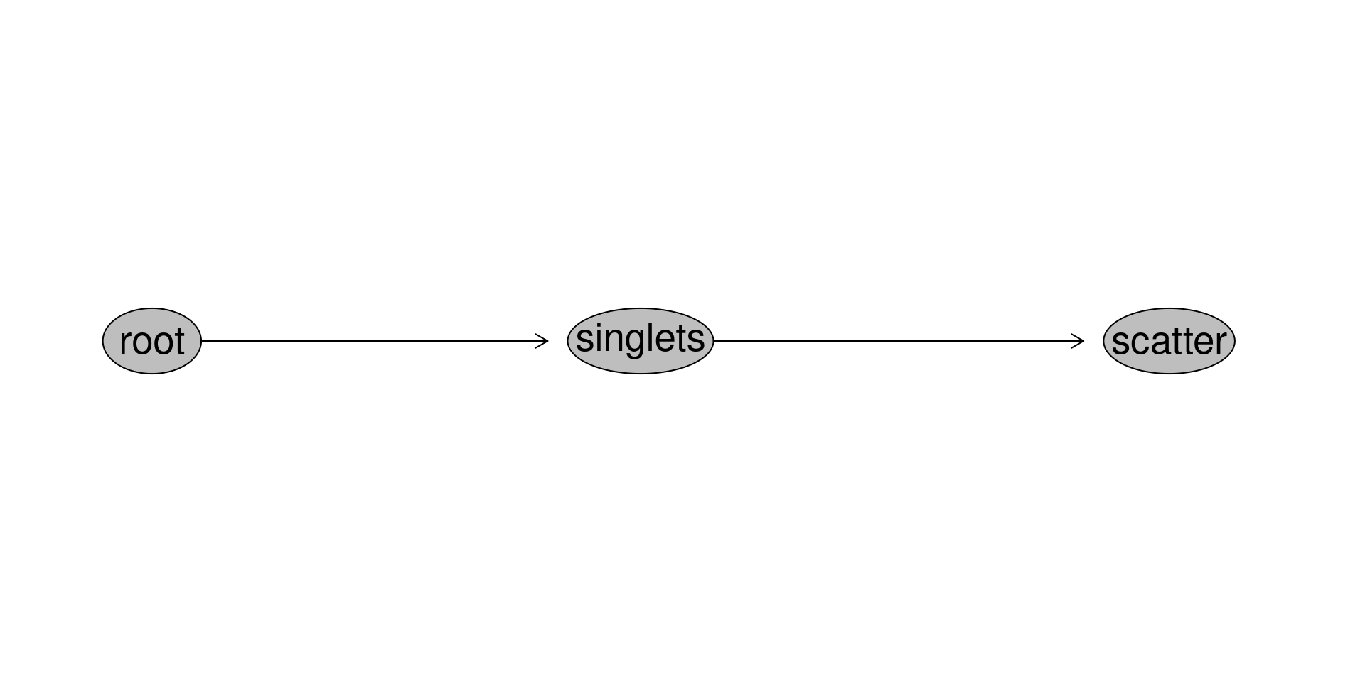
.
And with these bits of information gatherered, we can proceed with extracting the data for the gated region
ExternalNegativeCytoSet <- gs_pop_get_data(CellsUnstained_GatingSet[1], "scatter", inverse.transform=TRUE)
ExternalNegativeMatrix <- exprs(ExternalNegativeCytoSet[[1]]) #[[1]] used to remove list item, allowing access
ExternalNegativeData <- data.frame(ExternalNegativeMatrix, check.names=FALSE)
head(ExternalNegativeData, 3)
Time UV1-A UV2-A UV3-A UV4-A UV5-A UV6-A UV7-A
1 438622 831.9593 778.8554 320.6302 551.5653 951.2559 1669.570 2715.357
2 617037 163.1787 648.4011 251.9823 378.1972 571.3487 1285.795 2267.992
3 424351 635.5347 833.6690 439.0358 776.8467 905.7384 1508.549 2887.907
UV8-A UV9-A UV10-A UV11-A UV12-A UV13-A UV14-A UV15-A
1 2032.371 1769.0094 800.2003 418.2853 232.27344 462.01770 412.1862 -263.0648
2 1298.662 945.9752 458.0015 146.5932 224.09154 11.37962 -158.3447 343.0175
3 2246.274 1656.5549 741.4443 382.2132 48.56685 300.62338 861.5596 452.2003
UV16-A SSC-W SSC-H SSC-A V1-A V2-A V3-A V4-A
1 123.1652 697386.6 1040374 1209238 627.9626 2166.519 2809.125 3234.344
2 421.2599 645795.8 942471 1014406 463.3754 1444.369 1735.869 2216.637
3 296.0122 686219.9 1084433 1240266 416.8308 1597.543 2194.638 3067.281
V5-A V6-A V7-A V8-A V9-A V10-A V11-A V12-A
1 4540.319 4687.444 6048.969 4634.919 2650.931 3493.256 1727.000 574.8187
2 3559.600 3138.644 4048.412 3201.551 2358.193 2851.681 1528.381 757.8309
3 4041.194 4103.550 6072.000 4242.081 2972.200 4151.400 1921.494 1307.8315
V13-A V14-A V15-A V16-A FSC-W FSC-H FSC-A SSC-B-W
1 1112.4432 486.1317 956.03778 115.0873 704763.4 1521517 1787182 668472.4
2 855.9372 575.7122 63.24982 760.9938 656259.5 1308291 1430964 637367.3
3 1347.0879 899.4563 763.40045 573.0996 688062.9 1494703 1714083 667890.4
SSC-B-H SSC-B-A B1-A B2-A B3-A B4-A B5-A B6-A
1 918654 1023491.4 1983.5399 2176.785 3039.66 1960.530 1156.220 1281.995
2 635218 674778.7 917.0845 1277.315 1667.77 1163.045 1371.110 1025.895
3 814286 906423.0 1496.2996 2321.605 2595.19 1985.685 1749.475 1826.955
B7-A B8-A B9-A B10-A B11-A B12-A B13-A B14-A
1 964.1451 523.0545 1321.0598 156.84526 476.1246 -91.51968 102.2451 319.9955
2 892.5800 611.6502 400.0747 59.28042 399.4903 233.47961 104.3903 56.4847
3 1250.5350 551.4598 491.9849 443.88547 605.6055 195.19466 540.9299 467.8703
YG1-A YG2-A YG3-A YG4-A YG5-A YG6-A YG7-A
1 699.1604 1479.5896 1821.7504 1275.4702 929.5995 678.44000 350.2801
2 1048.1096 606.8998 698.9498 783.7895 645.3300 20.08974 1117.2704
3 1117.9000 968.3796 941.5695 1209.7404 567.4197 988.89050 1176.6302
YG8-A YG9-A YG10-A R1-A R2-A R3-A R4-A R5-A
1 753.40967 501.1998 448.4202 734.4401 745.4301 413.2798 148.2604 -17.98958
2 90.58011 345.4496 248.7099 181.4405 131.6699 101.9197 869.3303 -119.34999
3 607.80963 248.9898 -217.4903 629.3702 520.5204 523.2496 234.7096 165.12973
R6-A R7-A R8-A
1 334.5999 -642.38977 182.00024
2 229.3896 204.89000 590.10034
3 120.6796 -32.82967 41.78999.
With this done, we can remove the non-detector columns, summarize by median, and do the data tidying needed for the visualization.
ExternalNegativeDataSignature <- ExternalNegativeData[!stringr::str_detect(colnames(ExternalNegativeData), "FSC|SSC|Time")]

ExternalNegativeSignature <- ExternalNegativeDataSignature |> summarize_all("median")

ExternalNegativePlotData <- ExternalNegativeSignature |>
   mutate(Fluorophore="ExternalBackground") |> relocate(Fluorophore, .before=1)
.
And lets go ahead and combine in the data we have for the InternalNegative so we can do a direct comparison between them. Lets start off by first visualizing just the raw MFI values using VisualizeSignature()
.
As we can see, the external background signature is a little dimmer in terms of MFI compared to the internal controls raw signature values. Let’s check for the normalized signature.
.
As we can see, while the main autofluorescence peaks are similar, we do have some additive contribution to the red detectors for the internal negative compared to the external negative, likely due to a bit of underlying APC-Fire 810 staining occuring. Lets see how this would have impacted the overall signature.
InternalFluorophore <- PositiveSignature - NegativeSignature
InternalFluorophoreData <- InternalFluorophore |>
   mutate(Fluorophore="APCFire810minusInternal") |>relocate(Fluorophore, .before=1)

ExternalFluoruophore <- PositiveSignature - ExternalNegativeSignature
ExternalFluorophoreData <- ExternalFluoruophore |>
   mutate(Fluorophore="APCFire810minusExternal") |>relocate(Fluorophore, .before=1)

CombinedAPCFire810 <- bind_rows(InternalFluorophoreData, ExternalFluorophoreData)
.
At which point, visualizing difference in raw values for the background subtracted APC-Fire 810
.
We can see some minor differences present for the Violet detectors. Let’s check for the normalized signature
.
So for this particular antigen-Fluorophore combination, the overall signature didn’t change dramatically depending on whether we used the internal or external autofluorescence for background subtracction, outside some differences in the autofluorescence peak detectors (V8 and B3) due to the differences due to the external unstained being less bright compared with the internal unstained.
.
The differences that had observed between the unstained likely arising from non-specific staining in the red detectors ultimately didn’t seem to dramatically shift anything in the extracted fluorophore signature.
.
This is likely due to the actual positive signal present on those detectors for the single-color being substantially greater MFI to begin with than the little bit of non-specific signal present on the unstained cells, which although present was ultimately neglible at the time of subtraction.
.
As with everything in flow, this is for this particular fluorophore-antigen combination, on this particular specimen, and this pattern has no guarantees to hold up for other fluorophores (or even this same florophore on other experimental days). But it is a good illustration of the things to consider when carrying out the process of characterizing a fluorescent signature from our unmixing controls.
Signatures by Percentiles
.
Having now had some experience with the basic mechanics of extracting fluorescent signatures (after subtracting out either internal or external background), let’s carry out one of my time-honored traditions, going down a rabbit-hole!
.
When I was first learning how to unmix back in late 2021, I was always curious how placing a gate on the positive peak just 1 mm to the left or right might affect the unmixing result. Unfortunately, short of rather tedious re-unmixing, there was no easy way to answer this question at the time.
.
With our exisiting code above, we could obviously attempt to implement something similar using flowGate, however, we could also take a different approach. This would be for our gated region, we could separate on basis of the peak detector cells based on their MFI into a series of percentile bins. By looking across these 10% (or whatever range bins), we could repeat the process above for fluorescent signature extraction, and visualize the differences that occur.
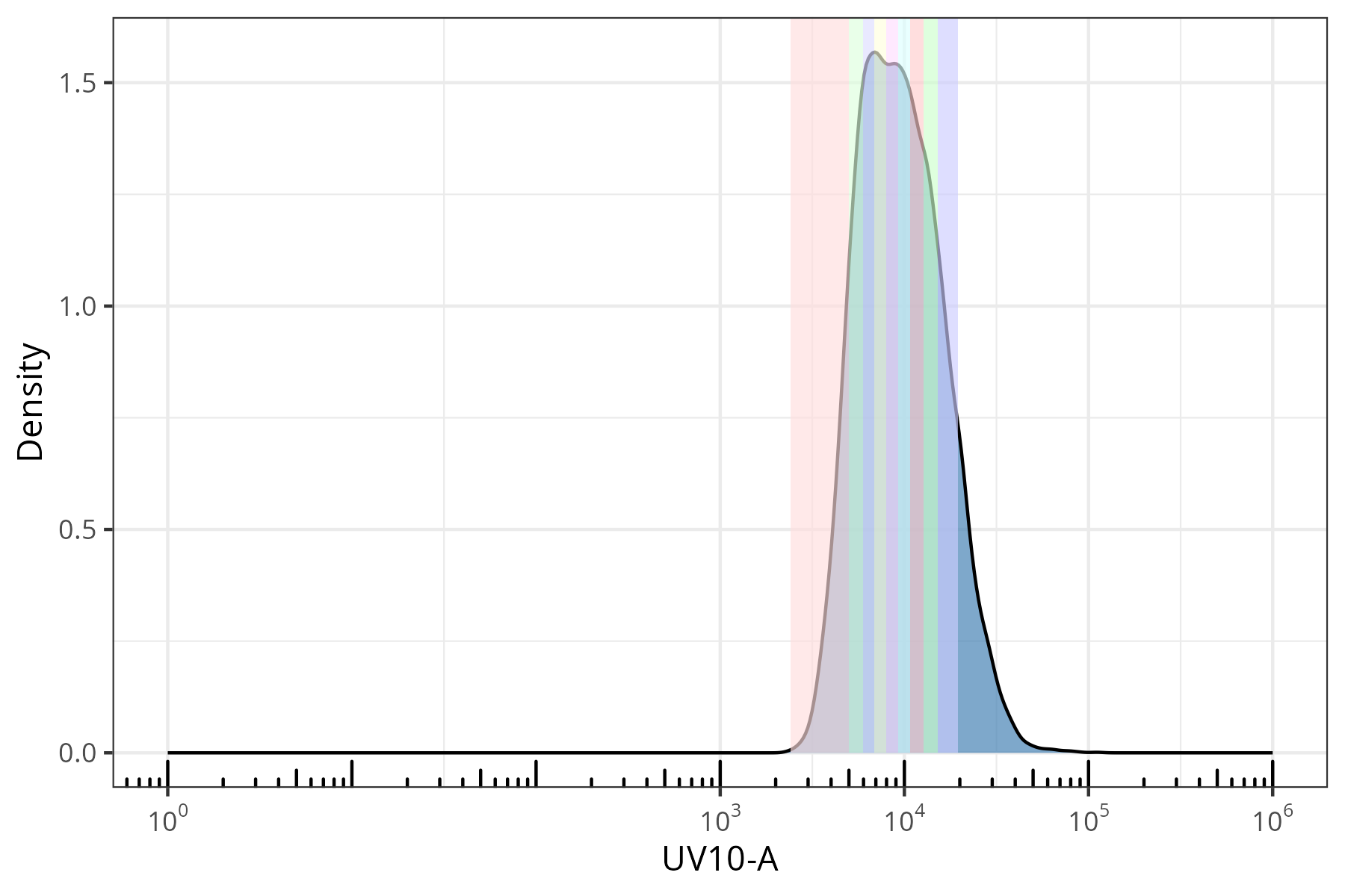
.
As there are multiple moving pieces, the code to do the above is part of the Luciernaga_LinearSlices() function from Luciernaga. However, since the implementation can be rather fine-tuned, it is not great to suddenly introduce towards the end of a walk-through.
.
We will rely on the LuciernagaIntegration() wrapper function to instead pass the contents of a particular gate to Luciernaga, and return the corresponding data.frames and plots that we might be interested in as a list object.
.
In addition to our GatingSet, we need to provide a pData template that also contains a Detector and Negative column to match the expected data.frame syntax, which we can do throyugh some data tidying with dplyr. Additionally, the particular fluorophore and particular gate name need to match. So we will use the gs_pop_set_name() function to rename our existing GatingSet gate to match the syntax by adding in a space. With that done, we can run the LuciernagaIntegration() wrapper, and save the list to a “APCFire810” variable object.
$`DTR_2023_ILT_01-Reference Group-DR_CD38 APC-Fire 810 (Cells).1235692.fcs`
NULL.
The return of this function is a list, with various data.frames and plots being retrieved for the cells in the gate in one go.
.
For this particular example, to compare across narrow slices of the positive peak, we will need to look at the LinearSlices_Plot. Lets see what effect gating in 10% bins across the R8-A detector would have had on the normalized fluorescent signature of our APC-Fire 810.
.
In this case, the primary peak (R8) remains the same. However, for the dimmer bins, we have a step-ladder appearence on the V7-A detector. This pattern is similar on the R1-A detector.
.
We showed similar data for our Cyto 2025 presentations, where we attributed this pattern to leftover residual autofluorescence, since not all cells are equally bright for autofluorescent molecules. When gating for dimmer cells, while the peak-detector remains the same, any residual autofluorescence leftover after the background subtraction makes up a greater proportion of the signature compared to the brighter staining cells, where the residual autofluorescence contribution is particularly neglible. This in turn results in the step-ladder appearance that we end up seeing on the autofluorescence detectors.
.
When this residual is substantial, it can substantially impact unmixing, which is why for the final unmixing of this panel, we had to replace BUV615 CCR4 and PE-Cy5 CD25 cell controls with single-stained beads to address some of the unmixing issues that were encountered.
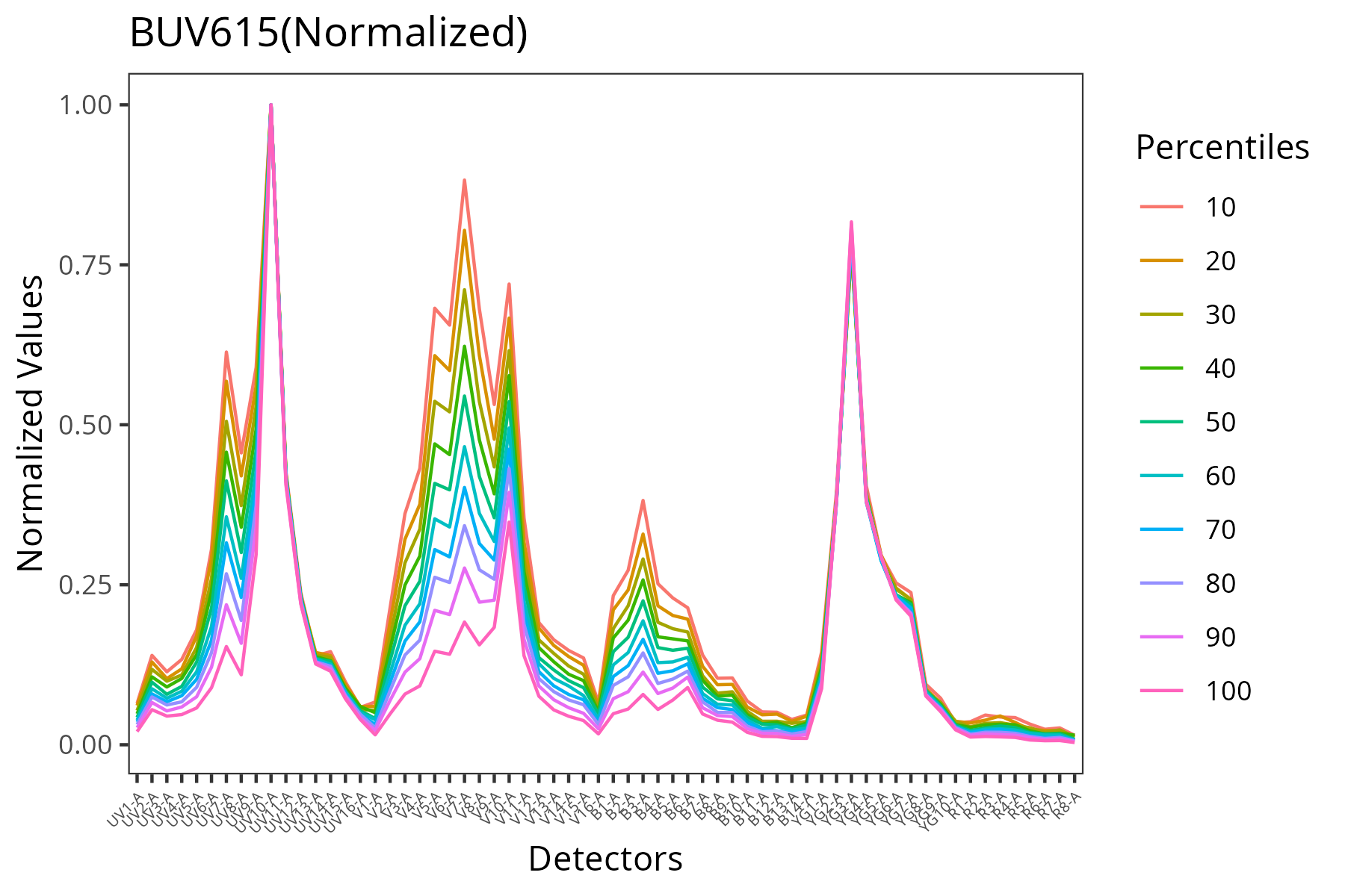
Single-Color Signatures from Individual Cells
.
So far, when looking at normalized fluorescent signatures, these have been on the basis of a gated region of cells that were positive for a particular marker (or further subdivided into 10% brighness bins in the case of the last example). Both of these approaches functions essentially the same, with the median measurement of those cells taken across each detector to derive the signature values.
.
However, there is also value in looking beyond the average signature, and seeing what information can be gleaned from the normalized signatures of individual cells. Within Luciernaga, various functions that are needed to orchestrate this are present (primarily via the LuciernagaQC() function).
.
The way this works in practice, is individual cells that have a primary peak detector for the staining fluorophore have the autofluorescent background subtracted. At this point, the individual cells signature is normalized, the peaks identified, and then cells that have normalized signatures at the same locations, of relatively similar heights end up grouped together, outputted as either summary data.frame or subsetted .fcs files that only contain cells with the same fluorescent signature (just differing by brightness)
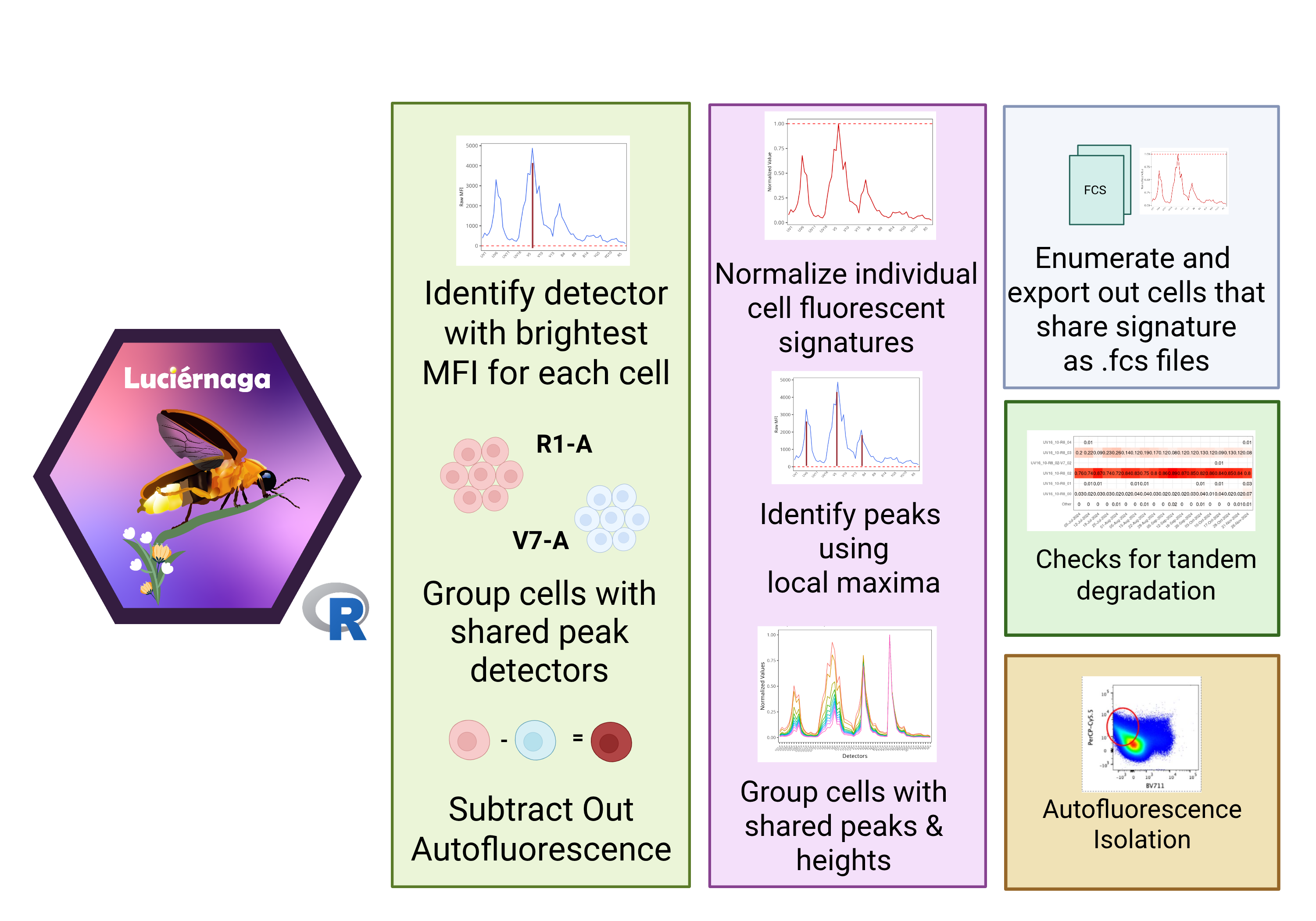
.
For now, rather than implement each plot separately, we will rely on the the LuciernagaIntegration() wrapper function. This returned list includes both the underlying data.frame and pots, so we can quickly glean information about the fluorescent signatures of individual cells that might otherwise be lost in the average signature.
.
Diving further into the returned list object, we can visualize all the identified normalized fluorescent signatures for our gated region of the APC-Fire 810 cell single-color control.
.
Unlike the previous characterization approaches, we end up with a lot more substantial variance for our normalized signatures from this APC-Fire 810 fluorophore. This is primarily manifested by the step-ladder like appearance for both the YG4 and R1 detectors. These were the same detectors that were unaccounted for when comparing the background subtracted signatures vs. those from the reference library.
.
So what is going on with this cell single-color control? Well, lets pull up the APC-Fire 810 reference signature, as well as that of the parent fluorophore APC which is part of the tandem dye.
.
So it turns out, the peak detectors for APC are both R1 and YG4. Therefore, for this particular single-color control, the deviations we have been seeing in the overall normalized signature is being drived partly by tandem degradation from APC-Fire 810 back to APC. This is clearly not complete, as R8 remains the primary detector, but there is a gradient of co-expression on the surface of individual cells which is contributing to the step-ladder pattern we are seeing.
.
So while visually striking, we need to know to what extent is this occuring. We can check the Luciernaga proportion plots which will display the proportion on a ggplot2 heatmap grid based on the individual signature variant.
.
Referencing the APC-Fire 810 signature, there shouldn’t be all that much signal on R1 or R2. However, from our proportion plot, we see that for a lot of cells in our gated region, the APC-Fire 810 variant signatures have greater amounts of R1/R2 present. Those with a R1/R2 detector measurement under 0.3 of the R8 detector are less than 2%. Around 72% of the cells have R1/R2 detectors values between 0.4 and 0.5, and then the other 25% of cells have substantial amounts of fully-degraded APC present on the surface of these individual cells.
.
When we step back and think about it, antibody-fluorophores exposed to reactive oxygen species may degrade individually rather than at the whole vial level. So at the cell surface, for highly expressed antigens, some will be bound by intact APC-Fire 810, while others may still end up bound by an antibody with only APC present. The balance between is what ends up being reflected in terms of the height of the R1/R2 peak, which is what is being captured by the grouping of individual cells by their normalized cell signatures.
.
So for this cell single-color control, the impact seems to be widespread. If we want to see how the proportion of the relative signature variants contributes towards the overall signature (ala what we would have seen by taking the averaged), we can check the AmalgamatedPlot output (Luciernaga_Amalgamate())
.
So in terms of the overall signature, still substantially different enough from the reference APC-Fire 810 to affect the comparison, but not as impacted by the cells that have heavily degraded down to APC to the point of being nearly the same height as the APC-Fire 810 peak (ex. R8-10_R2-09_YG4_05).
.
We will prelude next weeks topic by visualizing a cosine matrix, to get an idea of how different these individual signature variants are from each other (and start the imagine the amount of spreading/loss marker resolution/overcalculating APC fraction that might be occuring at the time of unmixing).
Autofluorescence Signatures from Individual Cells
.
In the example above, we saw an useful use case of characterizing cell single-color controls on the basis of their individual cell signatures in order to identify tandem degradation. But at that point, you might be wondering, can we use the same tools to characterize autofluorescence signatures (and maybe even export them out for use as reference signatures for unmixing). Why yes, we can.
.
Let’s go ahead and load back in our saved intermediate for the CellUnstained.gs
.
With this done, we will need to create a modified template to mimic what we had for the cell single controls to be able to utilize the LuciernagaIntegration() wrapper. We will need to remembber to set the “Unstained” argument to TRUE in order to skip the background subtraction step entirely.
.
After LuciernagaIntegration() finishes its run, we can querry the returned list for the returned data.frames and plots individually. For the plots, we can again use the plotly packages ggplotly() function for more interpretability via the interactive elements.
.
Starting off, lets see whether if we had broken the gating region into bins of 10% based on the UV7-A detector brightness whether we would have seen much difference in the normalized signature
.
Similar to what we saw with APC-Fire 810, this approach didn’t induce much signature variation, outside slightly higher peaks for V7 and B3.
.
Let’s go ahead and check what the LuciernagaQC() output returned as far as grouped individually normalized signatures returned.
.
As is immediately apparent, everything appears a bit fuzzy! Although most of the variation is around the UV7-A and B3-A detectors. In everyday practice, if we unmixed using a unstained signature that didn’t capture this variability, for those cells that did fit those patterns would end unmixing incorrectly (and fluorophores that had contributions with those detectors would end up similarly affected).
.
Lets go ahead and check the proportion plot output, to help determine which of these fuzzy signatures retrieved from our gating region make up a subtantial proportion of cells, and which ones might be rare enough to pass over.
.
Glancing at the data, V7 peak (1.0), B3 (0.5 of peak, ~50%), UV8 (0.4 of peak, ~ 40%) was the signature of 27% of the cells within our gated region. This was followed by adjacent signatures for V7 peak (1.0), B3 (0.6), UV8 (0.4) at 16%, and V7 peak (1.0), B3 (0.5), UV8 (0.3) that only differed by a slightly brighter or dimmer bin.
.
While cells with signatures where the secondary UV8 peak was higher than the B3 peak were present, for INF052 they were relatively rare not making up a substantial portion of the individual cell signatures. This is not always the case for CBMC, which led to this Cyto 2025 poster where we looked at what effect these variants had on unmixing.
.
Lets go ahead and visualize how these proportions when averaged would impact the overall fluorescent signature. Checking the amalgamated plot, we can see the peaks shared by the unstained signatures, as well as where substantial variance is present.
.
Please note, in our experience, some of the quirkier unmixing errors that we encounter are often tied to those individual cells having autofluorescences in the UV8 or B3 regions that don’t follow what other cells are doing. Since unmixing occurs at the individual cell level, these can matter as we will see in two weeks for the unmixing walk-through.
.
And previewing next time, lets see how these cell signatures differ from each other in terms of cosine value (i.e. similarity for those who speak Cytek Aurora)
.
Not just a single autofluorescence signature after all it turns out, no wonder some specimens have odd unmixing patterns for random small cell populations.
Signature Matrices
.
Today in this primary course material, we did a thorough walk-through of the process by which we can extract normalized fluorescent signatures from our unmixing controls (both single-colored and unstained). However, as is not lost to many of you, we did this for just a single fluorophore, and have 28 remaining to go. Do we need to repeat all the above code for each???
.
One option would be to try to scale-up, repeating the gating process acrooss the individual single-color controls, before breaking out flowGate to write a template to create fluorophore-specific positive gates on the correct detector based on their respective single-color control within the GatingSet. It would be a pain to write out all that code the first time around, but it could be used. Subsequently, after we extract the signatures, we could cobble them together to get to signature matrix we would need for unmixing.
.
However, that process as described above, sound more painful than it needs to be, especially when we have the power to write functions that can mediate all these steps we would need to implement for us behind the scenes. You can see how the new flowGate and Luciernaga functions were used to make our lives way way way easier in the bonus walkthorugh for Signature Matrices.
.
The signature matrices from this bonus walk-through can be found below. For cells
                      name              Fluorophore Antigen  Type Detector
1           PBMC_Unstained           PBMC_Unstained         Cells
2  PBMC_Monocyte_Unstained  PBMC_Monocyte_Unstained         Cells
3 PBMC_Activated_Unstained PBMC_Activated_Unstained         Cells
                  Negative UV1-A UV2-A UV3-A UV4-A UV5-A UV6-A UV7-A UV8-A
1           PBMC_Unstained 0.046 0.087 0.075 0.095 0.146 0.251 0.537 0.405
2  PBMC_Monocyte_Unstained 0.064 0.132 0.111 0.131 0.181 0.301 0.578 0.418
3 PBMC_Activated_Unstained 0.048 0.090 0.077 0.098 0.146 0.248 0.522 0.395
  UV9-A UV10-A UV11-A UV12-A UV13-A UV14-A UV15-A UV16-A  V1-A  V2-A  V3-A
1 0.372  0.151  0.092  0.056  0.044  0.054  0.041  0.035 0.076 0.258 0.434
2 0.381  0.150  0.089  0.052  0.042  0.049  0.036  0.029 0.089 0.300 0.485
3 0.364  0.152  0.093  0.058  0.047  0.056  0.043  0.037 0.076 0.257 0.427
   V4-A  V5-A  V6-A V7-A  V8-A  V9-A V10-A V11-A V12-A V13-A V14-A V15-A V16-A
1 0.505 0.768 0.730    1 0.746 0.527 0.609 0.350 0.204 0.195 0.180 0.164 0.097
2 0.532 0.769 0.728    1 0.757 0.536 0.609 0.341 0.191 0.176 0.155 0.136 0.076
3 0.500 0.761 0.725    1 0.750 0.530 0.606 0.344 0.199 0.189 0.172 0.155 0.090
   B1-A  B2-A  B3-A  B4-A  B5-A  B6-A  B7-A  B8-A  B9-A B10-A B11-A B12-A B13-A
1 0.248 0.302 0.418 0.284 0.248 0.201 0.148 0.110 0.118 0.075 0.058 0.054 0.045
2 0.253 0.305 0.425 0.302 0.262 0.218 0.163 0.118 0.123 0.076 0.057 0.050 0.040
3 0.247 0.306 0.427 0.290 0.254 0.205 0.153 0.114 0.121 0.078 0.060 0.056 0.046
  B14-A YG1-A YG2-A YG3-A YG4-A YG5-A YG6-A YG7-A YG8-A YG9-A YG10-A  R1-A
1 0.058 0.128 0.128 0.158 0.145 0.112 0.101 0.121 0.056 0.050  0.031 0.039
2 0.048 0.146 0.141 0.180 0.162 0.120 0.106 0.126 0.056 0.047  0.028 0.038
3 0.058 0.125 0.122 0.141 0.133 0.104 0.096 0.118 0.057 0.052  0.032 0.039
   R2-A  R3-A  R4-A  R5-A  R6-A  R7-A  R8-A
1 0.049 0.051 0.054 0.031 0.028 0.028 0.017
2 0.045 0.047 0.045 0.031 0.024 0.025 0.015
3 0.050 0.053 0.055 0.035 0.030 0.031 0.019.
And for beads
                                                                name
1 DTR_2023_ILT_00-Reference Group-DR_CCR4 BUV615 (Beads).1237096.fcs
2  DTR_2023_ILT_00-Reference Group-DR_CCR6 BV786 (Beads).1237097.fcs
3  DTR_2023_ILT_00-Reference Group-DR_CCR7 BV650 (Beads).1237098.fcs
  Fluorophore Antigen  Type Detector      Negative UV1-A UV2-A UV3-A UV4-A
1      BUV615    CCR4 Beads     UV10 BeadUnstained 0.007 0.031 0.025 0.021
2       BV786    CCR6 Beads      V15 BeadUnstained 0.000 0.000 0.002 0.001
3       BV650    CCR7 Beads      V11 BeadUnstained 0.000 0.000 0.003 0.002
  UV5-A UV6-A UV7-A UV8-A UV9-A UV10-A UV11-A UV12-A UV13-A UV14-A UV15-A
1 0.021 0.023 0.016 0.007 0.207  1.000  0.397  0.211  0.121  0.107  0.066
2 0.002 0.002 0.001 0.001 0.001  0.000  0.000  0.000  0.002  0.042  0.155
3 0.002 0.002 0.002 0.001 0.001  0.032  0.169  0.078  0.056  0.045  0.026
  UV16-A  V1-A  V2-A  V3-A  V4-A  V5-A  V6-A  V7-A  V8-A  V9-A V10-A V11-A
1  0.035 0.000 0.001 0.001 0.001 0.002 0.002 0.003 0.018 0.103 0.281 0.094
2  0.126 0.053 0.054 0.051 0.022 0.010 0.006 0.006 0.003 0.002 0.003 0.003
3  0.015 0.064 0.067 0.062 0.026 0.011 0.007 0.006 0.005 0.024 0.300 1.000
  V12-A V13-A V14-A V15-A V16-A B1-A B2-A  B3-A  B4-A  B5-A  B6-A  B7-A  B8-A
1 0.049 0.028 0.019 0.013 0.005    0    0 0.001 0.005 0.032 0.069 0.031 0.024
2 0.002 0.016 0.238 1.000 0.551    0    0 0.000 0.000 0.000 0.000 0.000 0.000
3 0.444 0.320 0.194 0.122 0.047    0    0 0.000 0.000 0.001 0.003 0.012 0.008
   B9-A B10-A B11-A B12-A B13-A B14-A YG1-A YG2-A YG3-A YG4-A YG5-A YG6-A YG7-A
1 0.021 0.009 0.006 0.005 0.003 0.002 0.089 0.471 0.999 0.449 0.339 0.254 0.222
2 0.000 0.000 0.002 0.009 0.020 0.023 0.000 0.000 0.000 0.000 0.000 0.000 0.001
3 0.007 0.004 0.002 0.002 0.001 0.001 0.001 0.003 0.026 0.209 0.133 0.101 0.110
  YG8-A YG9-A YG10-A  R1-A  R2-A  R3-A  R4-A  R5-A  R6-A  R7-A  R8-A
1 0.085 0.057  0.025 0.007 0.008 0.007 0.004 0.003 0.002 0.001 0.001
2 0.006 0.025  0.021 0.000 0.000 0.000 0.001 0.007 0.033 0.090 0.050
3 0.039 0.025 0.012 0.124 0.122 0.103 0.068 0.046 0.026 0.023 0.010.
Ultimately, once we have these signature matrices, we can use them for signature comparisons (which we will go into next time) as well as leverage them to unmix raw full-stained samples (as we will cover in a couple weeks).
Take Away
.
Over the course of this walk-through, we started with the set up that was needed to clean up our GatingSets in order to get at the cells that would provide the best signatures without introducing additional interpretation challenges. From there, we learned how to retrieve the cytoset for the gated cells, retrieve the exprs matrix, and isolate out the fluorescent detectors.
.
At this point, we orchestrated our way through summarizing for median, background subtraction, and normalization. We additionally learned various new functions that can help us visualize the signatures (both raw and normalized) and used these to screen an APC-Fire 810 to get a better understanding of what is going on when we set up our experiments for unmixing. We also took advantage of the LuciernagaIntegration() wrapper in order to get some additional insight about tandem degradation and autoflorescence variation in our unmixing controls.
.
Overall, I hope this walk-through, despite its length, was helpful. And I would like to end on circling back to how it can help us re-contextualize what the community as a whole has through various means converged on in terms of best practices for singl-color unmixing controls.
.
- Single-color cells need to be as bright or brighter than the full-stained sample.
.
From our dividing things up by percentile, we did observe that antigen-fluorophores with dimmer staining have greater proprotion of residual autofluorescence contribution to the signatures.
.
Likewise, for APC-Fire 810, for the cells where more of the tandem has been degraded, the dimmer staining cells for that detector are likelier to have more APC present in the overall signature.
.
This still leaves open the question of why beads when only out to 10^4 when full-stained cells are at 10^6 unmix horridly in some cases, but that is for another day.
.
- Matching autofluorescences
.
As we saw, there can be substantial variation in terms of brightness and signature for cells even within one gated region. This makes sense in light of its not just one single biological molecule causing the autofluorescence signature, rather it is the combination of all of them that falls within certain signature shapes. Activate or add insult to these cells, and the relative ratio of these biomolecules shifts far enough, we end up with a new variant that may need to be accounted for.
.
Likewise, when not extracting out the corresponding amount of background, these leftover autofluorescence residuals can end up incorporated into the overall fluorophore signature, complicating analysis.
.
- Same Fluorophore
.
Beyond why no, we just can’t substitute in BV510 for Zombie Aqua, the observed variation we saw for APC-Fire 810 following tandem degradation opens a bunch of questions that we will tackle in the next couple sessions. Is it better to use the degraded tandem as is? Or provide a proper APC-Fire 810 signature? What if APC is also already present in the panel. More questions than answers, but fascinating none the less.
.
- Enough events
.
Clearly important part, given the fuzzyness of the individual cell normalized signatures. Likewise, cytometers are noisy, there are additional variation that is not due to biology, having sufficient events can smooth those sharp curves out.
.
We will revisit some of these points (and try to answer some of these questions) as we move through both the next two sessions, as well as the bonus content. Until then, thanks for persevering through my spectral signature nerd out. Next up, signature comparison and unmixing-dependent spreading!
Additional Resources
.
In general, due to the nature of the topic, for this section, the additional resources is kind of intermingled, so you will encounter both spectral signatures, comparisons and unmixing often in the same paper or talk. Here are a few of many exceptional resources tht I have found worthwile over the years.
.
Spectral cytometry have you feeling all mixed up? Let’s get unmixed! Peter Mage’s CytoBytes short explanation. His FlowTex talk from a couple years ago is also well worthwhile
.
Advanced Unmixing Laura Johnston covers some of the same concepts in this Aurora tutorial, but having walked through the examples above, it takes on a whole new light of things to consider.
.
A comparison of spectral unmixing to conventional compensation for the calculation of fluorochrome abundances from flow cytometric data One of David Novo’s papers, well worthwhile (although the math-panic is real on my end).
Take-home Problems
Problem 1
In the example above, we deep dived the APC-Fire 810 single-color control. Since this is just one of the 29-single colors in the panel, check the pData, identify a fluorophore and marker of interest and repeat the process detailed above for your selected fluorophore. Report whether your chosen fluorophore behaved similarly or otherwise in terms of fluorescent signature variants as was the case for APC-Fire 810.
Problem 2
For this example, we gated the positive cells according to the “as bright or brighter” guideline. But what would we have seen if we had included the rest of the positive staining cells? Using flowGate, adjust the gate to include the less bright cells, and report whether this affected the overall signature profiles for the APC-Fire 810 control.
Problem 3
An important part of retrieving the fluorescent signature is to subtract the background autofluorescence. This could vary based on donor, cell type or treatment condition. With the tools provided in this walkthrough, compare the autofluorescent signatures for the 3 cell unstained controls, and whether their use as background would have affected the overall APC-Fire 810 extracted signature or not.