10 - Downsampling and Concatenation
2026-04-28

![]()
![]()
For the YouTube livestream schedule, see here
For screen-shot slides, click here
Background
.
Welcome to the tenth week of Cytometry in R! This is the official start of the “Cytometry Core” section, which means we are one-third of the way through the course!
.
In the first section “Introduction to R”, we were primarily focused on building a solid foundation of R skills, while introducing the basic infrastructure components of working with flow cytometry files using the various Bioconductor packages. Consequently, a lot of the previous lessons revolved around providing solved code examples, and then walking through what they did line-by-line.
.
While this remains especially helpful for those starting off (which is vast majority of course participants), in every R journey, there is a point where we start going beyond copying-and-pasting code, and instead begin attempting to write our own code based on contextual understanding of where we are at, and what we are trying to do, relying on modifying code snippets that we remember previously encountering, repurposing them toward accomplish our new goal.
.
This gradual transition in approach is what I call “bulding a coding mindset”. With time and practice, you will notice going from verbalizing broad “I am going to do task XYZ” goals, towards approaching the problem more from the lense of “first break this overall task I want to accomplish into a series of steps, and complete these smaller goals in turn by applying previous knowledge and targeted google searches to fill in the gaps as I go.”
.
While this may seem daunting when applied to coding, for those of us coming from the lab-bench, it’s analogous to that point where instead of needing to constantly refer back to our printed lab protocol for each and every of the (countless) staining/wash steps, we instead started remembering the sequence of events in context of what was occuring for the cells in our tube/plate, gradually decreasing the need to refer back to the protocol.
.
With this in mind, my goal of this section is not to immediately shove you all off the deep-end of the pool only to watch you drown. Rather, we will continue building on the foundation you have been assembling, while providing additional supervised space to attempt your own ideas that may or not work. So the lesson formats will gradually shift to accomodate this move towards greater coding independence over the next 10 sessions.
.
For the next couple weeks, we will start off by building out some of the toolsets that will be very much needed for the high-dimensional and unsupervised analysis weeks. Continuing from where we left off last time with functions, we will cobble together various concepts we have previously encountered with the goal of being able downsample our .fcs files to a desired number (or percentage) of cells for a given cell population. Once this has been accomplished, we will explore how to concatenate these downsampled files together, before saving them to new .fcs files (while hopefully updating the metadata correctly so that commercial software can visualize them correctly).
Walk Through
Housekeeping
As we do every week, on GitHub, sync your forked version of the CytometryInR course to bring in the most recent updates. Then within Positron, pull in those changes to your local computer.
For YouTube walkthrough of this process, click here
After setting up a “Week10” project folder, copy over the contents of “course/10_Downsampling/data” to that folder. This will hopefully prevent merge issues next week when attempting to pull in new course material. Once you have your new project folder organized, remember to commit and push your changes to GitHub to maintain remote version control.
If you encounter issues syncing due to the Take-Home Problem merge conflict, see this walkthrough. The updated homework submission protocol can be found here
Why Downsample?
.
There are various reasons why we might want to downsample (subset our .fcs files to a certain number or percentage of cells), especially in context of unsupervised analysis.
.
Traditionally, one of the main ones is limited computational resources. Rapid Access Memory (RAM) was often in limited quantity, especially compared to the size of .fcs files. When working with a large dataset, downsampling allowed for more equal representation across all acquired files to be accounted for in the subsequent analysis phase, without maxing out the available RAM and triggering the software to crash out due to lack of memory. This is particularly the case for some unsupervised clustering and dimensionality reduction algorithms, that are trying to differentiate how similar or different all the cells within the analysis are from each other.
.
Separately, some statistical analysis methods primarily rely on counts. Unlike frequency, which partially standardizes the comparison by leveraging against the parent gate, methods that rely on counts for their statistic may be similarly assisted when a defined number of cells at a designated gate are utilized.
.
Regardless of reason, we will need to figure out a few logistics when implementing a down-sampling strategy in R. We will first figure out the process using a single specimen, leveraging what we learned within the GatingSet lesson to be able to specify our gate of interest, and then leverage the resulting code to implement a function that can be used to iterate through all the files within the gating set.
Setup
Load .fcs files
.
Before we can downsample, we will need to have our .fcs files brought into R. We consequently repeat the loading in process that we have been seeing fairly regularly throughout the first section. This week, we will be working with some “larger” spectral .fcs files (since we will need to downsample). We are still limited by GitHub’s cap on max file size (5 MB), so if you want to use your own data, please feel free to substitute in the file path to your own .fcs files storage location.
#StorageLocation <- file.path("course", "10_Downsampling", "data") # Interacting directly
StorageLocation <- file.path("data") #For Quarto Rendering

fcs_files <- list.files(StorageLocation, pattern=".fcs", full.names=TRUE)
SFC_cytoset <- load_cytoset_from_fcs(fcs_files, truncate_max_range = FALSE, transformation = FALSE)
SFC_GatingSet <- GatingSet(SFC_cytoset)
SFC_Parameters <- colnames(SFC_GatingSet)
FluorophoresOnly <- SFC_Parameters[!stringr::str_detect(SFC_Parameters, "FSC|SSC|Time")]

Biexponential <- flowjo_biexp_trans(channelRange=4096, maxValue=262144,
     pos=4.5, neg=2, widthBasis=-500)
MyBiexTransform <- transformerList(FluorophoresOnly, Biexponential)
transform(SFC_GatingSet, MyBiexTransform)
A GatingSet with 3 samplesGate
.
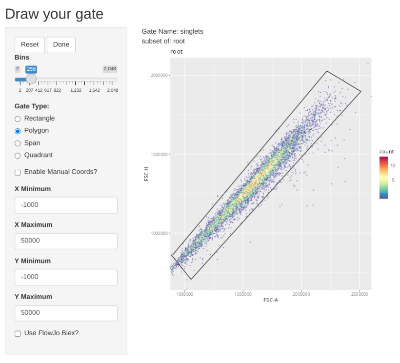
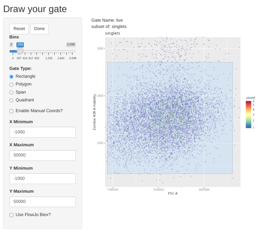
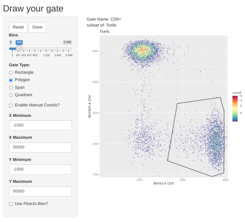
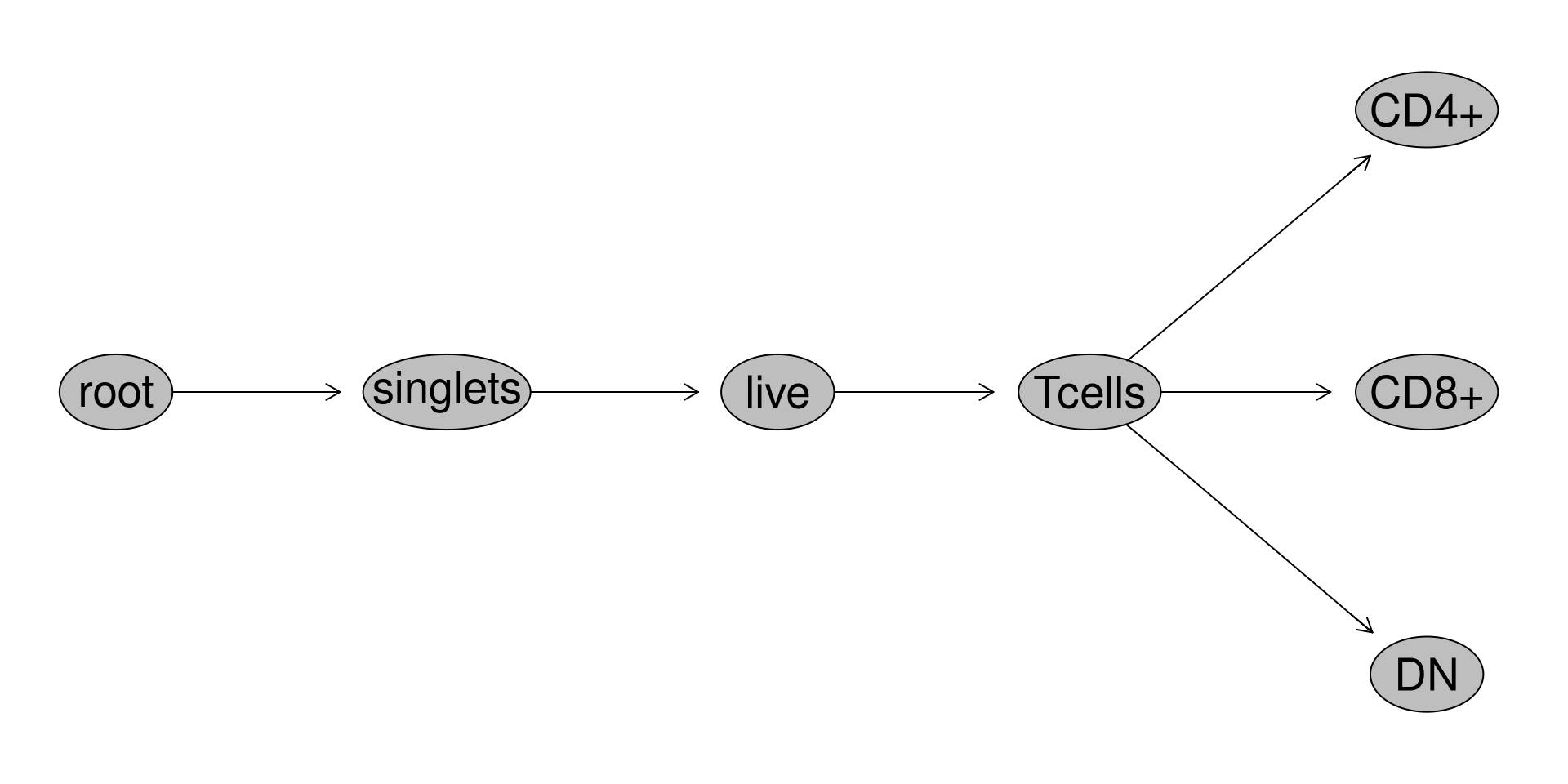
Once our data is in a GatingSet, we can add some general gates for the subsets using the flowGate package
GatingTable <- tibble::tribble(
~filterId, ~dims, ~subset,
"singlets", list("FSC-A", "FSC-H"), "root",
"live", list("FSC-A", "Zombie NIR-A"), "singlets",
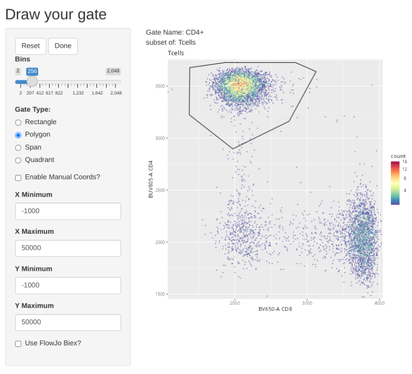
"Tcells", list("CD3", "CD45"), "live",
"CD4+", list("CD8", "CD4"), "Tcells",
"CD8+", list("CD8", "CD4"), "Tcells",
"DN", list("CD8", "CD4"), "Tcells",
)

Retrieving Counts
.
Let’s quickly check to see what specimens we will be working with for this dataset.
                                                                                                   name
2025_07_26_AB_02-INF052-00_Ctrl_Unmixed__Tcells.fcs 2025_07_26_AB_02-INF052-00_Ctrl_Unmixed__Tcells.fcs
2025_07_26_AB_02-INF100-00_Ctrl_Unmixed__Tcells.fcs 2025_07_26_AB_02-INF100-00_Ctrl_Unmixed__Tcells.fcs
2025_07_26_AB_02-INF179-00_Ctrl_Unmixed__Tcells.fcs 2025_07_26_AB_02-INF179-00_Ctrl_Unmixed__Tcells.fcs
.
We have so far gated for the three main T cell populations in cord blood (CD4+, CD8+ and Double-Negative (CD4-CD8-)). Considering that in cord blood mononuclear cells, the abundance of these subsets may vary a bit by donor, we want to make sure we downsample a number of cells that will result in each individual specimen providing a relatively similar contribution of cells to the final .fcs file we end up creating.
.
Looking at our retrieved data, the gate names are showing up as full file.paths.
 [1] "/singlets"                  "/singlets/live"
 [3] "/singlets/live/Tcells"      "/singlets/live/Tcells/CD4+"
 [5] "/singlets/live/Tcells/CD8+" "/singlets/live/Tcells/DN"
 [7] "/singlets"                  "/singlets/live"
 [9] "/singlets/live/Tcells"      "/singlets/live/Tcells/CD4+"
[11] "/singlets/live/Tcells/CD8+" "/singlets/live/Tcells/DN"
[13] "/singlets"                  "/singlets/live"
[15] "/singlets/live/Tcells"      "/singlets/live/Tcells/CD4+"
[17] "/singlets/live/Tcells/CD8+" "/singlets/live/Tcells/DN"
.
Let’s abbreviate them for simplicity using the basename() function.
                                                   name Population
                                                 <char>     <char>
 1: 2025_07_26_AB_02-INF052-00_Ctrl_Unmixed__Tcells.fcs   singlets
 2: 2025_07_26_AB_02-INF052-00_Ctrl_Unmixed__Tcells.fcs       live
 3: 2025_07_26_AB_02-INF052-00_Ctrl_Unmixed__Tcells.fcs     Tcells
 4: 2025_07_26_AB_02-INF052-00_Ctrl_Unmixed__Tcells.fcs       CD4+
 5: 2025_07_26_AB_02-INF052-00_Ctrl_Unmixed__Tcells.fcs       CD8+
 6: 2025_07_26_AB_02-INF052-00_Ctrl_Unmixed__Tcells.fcs         DN
 7: 2025_07_26_AB_02-INF100-00_Ctrl_Unmixed__Tcells.fcs   singlets
 8: 2025_07_26_AB_02-INF100-00_Ctrl_Unmixed__Tcells.fcs       live
 9: 2025_07_26_AB_02-INF100-00_Ctrl_Unmixed__Tcells.fcs     Tcells
10: 2025_07_26_AB_02-INF100-00_Ctrl_Unmixed__Tcells.fcs       CD4+
11: 2025_07_26_AB_02-INF100-00_Ctrl_Unmixed__Tcells.fcs       CD8+
12: 2025_07_26_AB_02-INF100-00_Ctrl_Unmixed__Tcells.fcs         DN
13: 2025_07_26_AB_02-INF179-00_Ctrl_Unmixed__Tcells.fcs   singlets
14: 2025_07_26_AB_02-INF179-00_Ctrl_Unmixed__Tcells.fcs       live
15: 2025_07_26_AB_02-INF179-00_Ctrl_Unmixed__Tcells.fcs     Tcells
16: 2025_07_26_AB_02-INF179-00_Ctrl_Unmixed__Tcells.fcs       CD4+
17: 2025_07_26_AB_02-INF179-00_Ctrl_Unmixed__Tcells.fcs       CD8+
18: 2025_07_26_AB_02-INF179-00_Ctrl_Unmixed__Tcells.fcs         DN
                   Parent Count ParentCount
                   <char> <int>       <int>
 1:                  root  9485       10000
 2:             /singlets  9253        9485
 3:        /singlets/live  8871        9253
 4: /singlets/live/Tcells  5680        8871
 5: /singlets/live/Tcells  2473        8871
 6: /singlets/live/Tcells   560        8871
 7:                  root  9549       10000
 8:             /singlets  9193        9549
 9:        /singlets/live  8517        9193
10: /singlets/live/Tcells  5147        8517
11: /singlets/live/Tcells  3028        8517
12: /singlets/live/Tcells   240        8517
13:                  root  9466       10000
14:             /singlets  9177        9466
15:        /singlets/live  8644        9177
16: /singlets/live/Tcells  6765        8644
17: /singlets/live/Tcells  1658        8644
18: /singlets/live/Tcells   129        8644
.
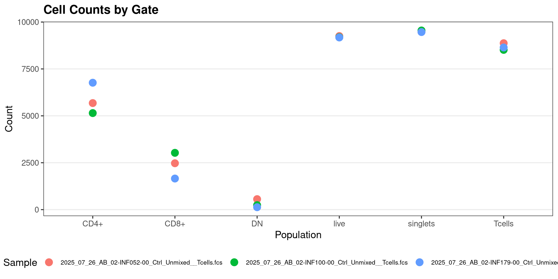
With this bit of cleanup done, lets plot them with ggplot2
Plot <- ggplot(Data, aes(x = Population, y = Count, color = name)) +
  geom_point(size = 4) +
  labs(
    title = "Cell Counts by Gate",
    x = "Population",
    y = "Count",
    color = "Sample"
  ) +
  theme_bw(base_size = 13) +
  theme(
    plot.title = element_text(face = "bold"),
    legend.position = "bottom",
    legend.text = element_text(size = 8),
    panel.grid.major.x = element_blank(),
    panel.grid.minor = element_blank()
  )
.
As we have encountered on a couple of the prior sessions, we can use the plotly package ggplotly() function to convert our static ggplot2 plots into interactive ones, which are useful in this context.
.
Looking at our gated T cell populations across specimens, we can see that in general, while each specimen has similar number of live T cells, there is a little more variability when it comes to the individual T cell subsets. We will revisit this later on as we build out the function logic.
Building Downsample
Broad Idea Sketch
.
Now that we have our dataset pre-requisites assembled within our local environment, lets start by planning out what we will need in order to assemble a downsampling function, at least in terms of inputs and what it will ideally return as outputs.
.
We are going to be starting off with our gated GatingSet, and similar to what we did during Week 09 with the CellConcentration() function, iterate through the individual GatingHierarchies using the purrr packages map() function.
.
Once an individual .fcs file ends up within our new function, we will need to extract out the exprs data (where measurements for individual cells are stored). From this original data, we will need to downsample (i.e. subset) a designated number of cells which correspond to individual rows (while also accounting for several possible exceptions we might encounter).
.
This modified exprs data then needs to be returned to the .fcs file, maintaining the rest of the parameter and description metadata intact so that it remains recognizable as a standard .fcs file. We would also want to be able to export out the .fcs file with modified name parameters so that we can distinguish the downsampled version from the original .fcs file, to avoid accidentally overwriting our original.
.
So, visualizing ahead, at the end of the iteration, we would end up with three new .fcs files, containing our target number of downsampled cells originating for our respective gate of interest.
.
With this rough sketch worked out, lets dive in.
Initial Skeleton
.
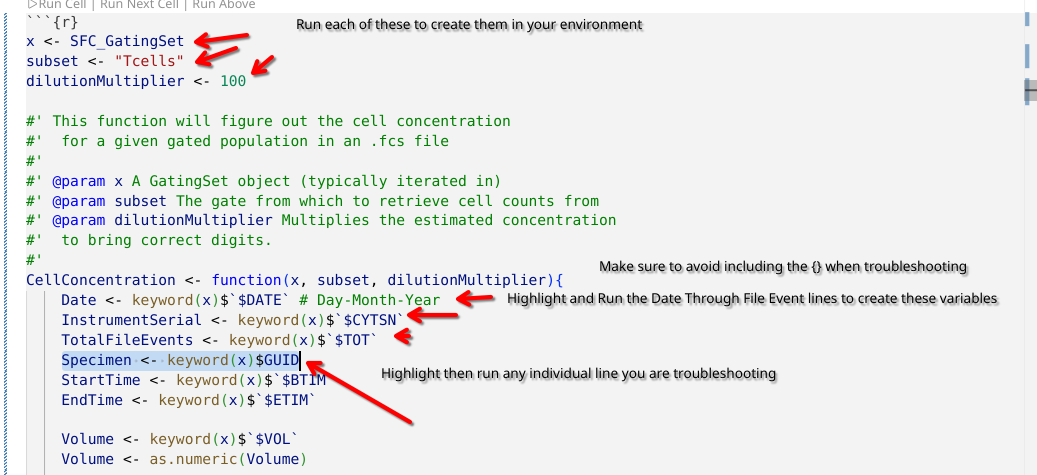
Getting started, lets go ahead and establish our initial function, as well as add elements of the roxygen2 skeleton for documentation. We will provide our first argument as “x”, which will serve as our standin for the individual .fcs file being iterated in via purrr.
.
When function building, highlighting and running (via Ctrl/Command + Enter) individual arguments being provided to the function can be helpful as you are writing it. These variables end up being created as objects in your environment (appearing under the variables tab in the right-secondary side-bar), and are available for use in troubleshooting and debugging. Here is an example of how highlight lines within the function that you want to run/troubleshoot would appear as.
.
Remembering back to last week, we remember that when we iterate a GatingSet object, we end up with a GatingHierarchy containing a single .fcs file, similar to if we had used [[]] on the GatingSet.
.
If we were to run the above code-chunk (resulting in “x” appearing in our created variables tab), by clicking on the class line in the chunk below, running Ctrl/Command + Enter would be the equivalent of having entered the same line of code in your console
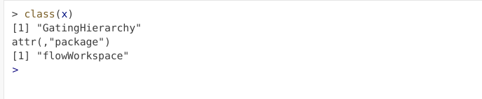
.
We can confirm that the object we are using for troubleshooting (x) is returning the same value as if we were iterating with purrr by setting the iteration to thefirst object (i.e. [1]) in our GatingSet, and make sure that both approaches are returning a GatingHierarchy. If they are discrepant (one returning a GatingSet or a list), then we likely missed a set of [] somewhere.
.
In this case, both are returning the same class of object, so we have correctly set up our function and outside argument standins correctly. Lets proceed to modify our the internals.
.
From the entire .fcs file, we will need to subset out the underlying data corresponding to our gated population of interest. This is similar to the code we used last time for CellConcentration, so we can quickly relocate that code from the respective lesson, then copy-and-paste it into our new function within the {}.
.
One thing to remember, the code within the function is only able to see variables that we pass in to it, which is done via arguments (that are present within the “()” ). So to get gs_pop_get_data() to run successfully, we will need to add “subset” as Downsampling’s second argument, or we will not be able to isolate the data associated for our respective gate.
#' This function downsamples from a designated gate to our desired number
#' of cells, returning as a new .fcs file
#'
#' @param x A GatingSet object, typically iterated in.
#' @param subset The gate from which to retrieve cell counts from
#'
Downsampling <- function(x, subset){
  EventsInTheGate <- gs_pop_get_data(x, subset)
}
.
Having made a change to the function, we need to re-run the code-block above, so that the changes we have made to our function are reflected within our environment. Once this code-block has been rerun, if we check under the variables tab we can see the information detailed for our function has changed.
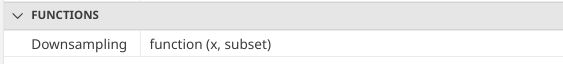
.
Likewise, if we run our function using our actual arguments, we can see that the returned object has now changed from returning the class() output we had as a placeholder to the returned ‘cytoset’ object from gs_pop_get_data()
[[1]]
A cytoset with 1 samples.

  column names:
    Time, SSC-W, SSC-H, SSC-A, FSC-W, FSC-H, FSC-A, SSC-B-W, SSC-B-H, SSC-B-A, BUV395-A, BUV563-A, BUV615-A, BUV661-A, BUV737-A, BUV805-A, Pacific Blue-A, BV480-A, BV570-A, BV605-A, BV650-A, BV711-A, BV750-A, BV786-A, Alexa Fluor 488-A, Spark Blue 550-A, Spark Blue 574-A, RB613-A, RB705-A, RB780-A, PE-A, PE-Dazzle594-A, PE-Cy5-A, PE-Fire 700-A, PE-Fire 744-A, PE-Vio770-A, APC-A, Alexa Fluor 647-A, APC-R700-A, Zombie NIR-A, APC-Fire 750-A, APC-Fire 810-A, AF-A

cytoset has been subsetted and can be realized through 'realize_view()'.
Accessing exprs
.
With our function building underway, gs_pop_get_data() returns to us a “cytoset object” of length 1. Remembering back during Week 03, we were able to use exprs() on a flowFrame object to retrieve the underlying MFI measurement data that we are interested in. Let’s try running it in this context and see if this will similarly work.
#' This function downsamples from a designated gate to our desired number
#' of cells, returning as a new .fcs file
#'
#' @param x A GatingSet object, typically iterated in.
#' @param subset The gate from which to retrieve cell counts from
#'
Downsampling <- function(x, subset){
  EventsInTheGate <- gs_pop_get_data(x, subset)
  MeasurementData <- exprs(EventsInTheGate)
}.
Judging by the error message, the exprs() function has no idea what do with a ‘cytoset’ object. With a little (or quite a lot) of investigation within the exprs help file and the flowWorkspace vignette, we see that the expected object being passed to the function is a mismatch for class, i.e. we are a level too high up in the hierarchy. Rather than passing a cytoset, we need to be at cytoframe level (individual object rather than a set) to successfully retrieve the exprs-associated data.
.
Fortunately, dropping down to an individual unit is similar to other list style objects, requiring us to modify the code by placing [[1]] next to our cytoset variable inside the function (EventsInTheGate). After updating the function (and re-running it), we can pass our data and check the output
#' This function downsamples from a designated gate to our desired number
#' of cells, returning as a new .fcs file
#'
#' @param x A GatingSet object, typically iterated in.
#' @param subset The gate from which to retrieve cell counts from
#'
Downsampling <- function(x, subset){
  EventsInTheGate <- gs_pop_get_data(x, subset)
  MeasurementData <- exprs(EventsInTheGate[[1]])
} Time SSC-W SSC-H SSC-A FSC-W FSC-H FSC-A SSC-B-W SSC-B-H
[1,] 88303 800625.8 412920 550990.7 745687.8 1207102 1500202 767241.9 336298
[2,] 151951 721600.7 522319 628176.2 713266.4 1364125 1621641 709783.5 365916
[3,] 225780 747106.5 305002 379781.6 678442.0 899363 1016943 694236.2 317438
SSC-B-A BUV395-A BUV563-A BUV615-A BUV661-A BUV737-A BUV805-A
[1,] 430036.5 2258.554 2967.613 1925.955 2098.853 3232.693 1879.053
[2,] 432868.6 2937.244 2664.265 2098.485 1966.986 3253.292 3515.342
[3,] 367294.9 3243.016 2398.396 2251.842 2118.144 3098.917 3549.486
Pacific Blue-A BV480-A BV570-A BV605-A BV650-A BV711-A BV750-A
[1,] 2059.758 2112.291 1701.588 3548.215 3713.888 2058.872 2508.425
[2,] 2120.267 2107.440 2218.929 3529.080 2071.707 2316.910 1962.467
[3,] 2179.407 2134.529 1849.710 3272.614 1848.897 1957.577 2104.743
BV786-A Alexa Fluor 488-A Spark Blue 550-A Spark Blue 574-A RB613-A
[1,] 1867.927 2302.473 3419.844 3225.375 2187.869
[2,] 2345.562 2223.587 3478.904 3267.592 2071.955
[3,] 1955.958 2390.761 3435.635 3201.560 2368.059
RB705-A RB780-A PE-A PE-Dazzle594-A PE-Cy5-A PE-Fire 700-A
[1,] 3421.698 2137.918 2676.039 2167.108 2276.323 3108.547
[2,] 3753.434 2118.650 2939.783 2391.270 2032.860 2862.195
[3,] 3299.392 2021.984 2868.770 2305.990 2083.745 2462.668
PE-Fire 744-A PE-Vio770-A APC-A Alexa Fluor 647-A APC-R700-A
[1,] 2156.676 1954.386 2203.288 2097.104 2124.087
[2,] 2188.545 2107.110 2056.971 2252.323 2084.971
[3,] 2227.207 1976.180 2335.905 2157.208 2105.890
Zombie NIR-A APC-Fire 750-A APC-Fire 810-A AF-A
[1,] 2319.684 3290.837 3289.486 2878.465
[2,] 2145.456 3337.221 3100.115 2868.599
[3,] 2191.646 3302.940 2974.669 2720.577.
Success, we have successfully retrieved the underlying data for T cells! (finally!)
.
But let’s quickly do a sanity check, and make sure that the numbers we are retrieving make sense. We can do this by adding summary() function to summarize the distribution for each of our MeasurementData columns.
#' This function downsamples from a designated gate to our desired number
#' of cells, returning as a new .fcs file
#'
#' @param x A GatingSet object, typically iterated in.
#' @param subset The gate from which to retrieve cell counts from
#'
Downsampling <- function(x, subset){
  EventsInTheGate <- gs_pop_get_data(x, subset)
  MeasurementData <- exprs(EventsInTheGate[[1]])
  summary(MeasurementData)
}[[1]]
Time SSC-W SSC-H SSC-A
Min. : 19 Min. : 668906 Min. : 99153 Min. : 149656
1st Qu.:223276 1st Qu.: 746226 1st Qu.: 374691 1st Qu.: 481748
Median :446601 Median : 765489 Median : 444238 Median : 567915
Mean :444126 Mean : 771548 Mean : 451345 Mean : 579404
3rd Qu.:664988 3rd Qu.: 787334 3rd Qu.: 514309 3rd Qu.: 657794
Max. :896504 Max. :1333696 Max. :2412543 Max. :3211955
FSC-W FSC-H FSC-A SSC-B-W
Min. :654257 Min. : 775895 Min. : 935556 Min. : 650346
1st Qu.:711727 1st Qu.:1159357 1st Qu.:1396508 1st Qu.: 727882
Median :724892 Median :1305759 Median :1585267 Median : 747608
Mean :725723 Mean :1296808 Mean :1570172 Mean : 754191
3rd Qu.:738849 3rd Qu.:1435574 3rd Qu.:1749781 3rd Qu.: 771752
Max. :821290 Max. :2040353 Max. :2428548 Max. :1430571
SSC-B-H SSC-B-A BUV395-A BUV563-A
Min. : 104214 Min. : 149874 Min. :1488 Min. :1113
1st Qu.: 310103 1st Qu.: 388649 1st Qu.:2561 1st Qu.:2732
Median : 361253 Median : 453426 Median :2926 Median :2997
Mean : 369627 Mean : 464231 Mean :2849 Mean :2966
3rd Qu.: 417589 3rd Qu.: 523766 3rd Qu.:3175 3rd Qu.:3225
Max. :2591438 Max. :3461184 Max. :3729 Max. :4049
BUV615-A BUV661-A BUV737-A BUV805-A Pacific Blue-A
Min. : 900.2 Min. :1361 Min. :1589 Min. :1413 Min. :1234
1st Qu.:1899.1 1st Qu.:1966 1st Qu.:2782 1st Qu.:2162 1st Qu.:2113
Median :2033.1 Median :2058 Median :3026 Median :3444 Median :2198
Mean :2058.7 Mean :2069 Mean :2921 Mean :2991 Mean :2193
3rd Qu.:2178.7 3rd Qu.:2154 3rd Qu.:3178 3rd Qu.:3525 3rd Qu.:2281
Max. :3471.2 Max. :3934 Max. :3567 Max. :3786 Max. :3413
BV480-A BV570-A BV605-A BV650-A BV711-A
Min. :1369 Min. :1430 Min. :1287 Min. :1185 Min. :1201
1st Qu.:2000 1st Qu.:1909 1st Qu.:3201 1st Qu.:2025 1st Qu.:1885
Median :2114 Median :2061 Median :3410 Median :2167 Median :2063
Mean :2157 Mean :2063 Mean :3359 Mean :2554 Mean :2056
3rd Qu.:2238 3rd Qu.:2209 3rd Qu.:3575 3rd Qu.:3528 3rd Qu.:2225
Max. :6763 Max. :3674 Max. :4020 Max. :4044 Max. :3571
BV750-A BV786-A Alexa Fluor 488-A Spark Blue 550-A
Min. :1531 Min. :1291 Min. : 934.2 Min. :3249
1st Qu.:2126 1st Qu.:1869 1st Qu.:2075.3 1st Qu.:3431
Median :2281 Median :2064 Median :2171.1 Median :3495
Mean :2284 Mean :2070 Mean :2187.6 Mean :3492
3rd Qu.:2435 3rd Qu.:2266 3rd Qu.:2280.9 3rd Qu.:3554
Max. :3187 Max. :3631 Max. :3333.9 Max. :3721
Spark Blue 574-A RB613-A RB705-A RB780-A PE-A
Min. :2966 Min. :1209 Min. :1566 Min. :1398 Min. : 771.5
1st Qu.:3160 1st Qu.:1950 1st Qu.:3292 1st Qu.:1947 1st Qu.:2267.5
Median :3222 Median :2139 Median :3579 Median :2080 Median :2499.5
Mean :3216 Mean :2234 Mean :3340 Mean :2085 Mean :2473.6
3rd Qu.:3276 3rd Qu.:2379 3rd Qu.:3706 3rd Qu.:2217 3rd Qu.:2695.1
Max. :3477 Max. :3877 Max. :4085 Max. :3596 Max. :3391.4
PE-Dazzle594-A PE-Cy5-A PE-Fire 700-A PE-Fire 744-A PE-Vio770-A
Min. :1451 Min. :1635 Min. :1695 Min. :1410 Min. :1559
1st Qu.:2098 1st Qu.:2072 1st Qu.:2689 1st Qu.:1969 1st Qu.:2059
Median :2224 Median :2173 Median :2889 Median :2076 Median :2184
Mean :2224 Mean :2287 Mean :2837 Mean :2120 Mean :2213
3rd Qu.:2353 3rd Qu.:2392 3rd Qu.:3043 3rd Qu.:2185 3rd Qu.:2330
Max. :3076 Max. :3661 Max. :3532 Max. :3742 Max. :4261
APC-A Alexa Fluor 647-A APC-R700-A Zombie NIR-A APC-Fire 750-A
Min. :1097 Min. :1356 Min. :1468 Min. :1735 Min. :1571
1st Qu.:2042 1st Qu.:1928 1st Qu.:2023 1st Qu.:2176 1st Qu.:3171
Median :2179 Median :2065 Median :2128 Median :2298 Median :3266
Mean :2184 Mean :2059 Mean :2133 Mean :2297 Mean :3226
3rd Qu.:2314 3rd Qu.:2194 3rd Qu.:2236 3rd Qu.:2421 3rd Qu.:3338
Max. :3838 Max. :3086 Max. :3153 Max. :2761 Max. :3609
APC-Fire 810-A AF-A
Min. :1692 Min. : 865.1
1st Qu.:2970 1st Qu.:2789.3
Median :3151 Median :2876.1
Mean :3044 Mean :2842.7
3rd Qu.:3249 3rd Qu.:2935.9
Max. :3538 Max. :3212.3 .
Looking at the distribution of the values for individual fluorophores, everything seems rather suspiciously in the same linear-style range to each other than what we would normally anticipate for spectral flow cytometry data.
.
We recall back to Week 07 that unlike many commerical softwares, transformations in R are applied directly to the underlying values. When we ran gs_pop_get_data, we did not specify that this transformation should be reversed, so we ended up retrieving the transformed data values.
.
We can correct this by setting the “inverse.transform” argument to “TRUE” within gs_pop_get_data(). After re-running the function, we get back
#' This function downsamples from a designated gate to our desired number
#' of cells, returning as a new .fcs file
#'
#' @param x A GatingSet object, typically iterated in.
#' @param subset The gate from which to retrieve cell counts from
#'
Downsampling <- function(x, subset){
  EventsInTheGate <- gs_pop_get_data(x, subset, inverse.transform=TRUE)
  MeasurementData <- exprs(EventsInTheGate[[1]])
  summary(MeasurementData)
}[[1]]
Time SSC-W SSC-H SSC-A
Min. : 19 Min. : 668906 Min. : 99153 Min. : 149656
1st Qu.:223276 1st Qu.: 746226 1st Qu.: 374691 1st Qu.: 481748
Median :446601 Median : 765489 Median : 444238 Median : 567915
Mean :444126 Mean : 771548 Mean : 451345 Mean : 579404
3rd Qu.:664988 3rd Qu.: 787334 3rd Qu.: 514309 3rd Qu.: 657794
Max. :896504 Max. :1333696 Max. :2412543 Max. :3211955
FSC-W FSC-H FSC-A SSC-B-W
Min. :654257 Min. : 775895 Min. : 935556 Min. : 650346
1st Qu.:711727 1st Qu.:1159357 1st Qu.:1396508 1st Qu.: 727882
Median :724892 Median :1305759 Median :1585267 Median : 747608
Mean :725723 Mean :1296808 Mean :1570172 Mean : 754191
3rd Qu.:738849 3rd Qu.:1435574 3rd Qu.:1749781 3rd Qu.: 771752
Max. :821290 Max. :2040353 Max. :2428548 Max. :1430571
SSC-B-H SSC-B-A BUV395-A BUV563-A
Min. : 104214 Min. : 149874 Min. :-2119 Min. : -5749
1st Qu.: 310103 1st Qu.: 388649 1st Qu.: 1871 1st Qu.: 2920
Median : 361253 Median : 453426 Median : 4889 Median : 5982
Mean : 369627 Mean : 464231 Mean : 7093 Mean : 9349
3rd Qu.: 417589 3rd Qu.: 523766 3rd Qu.:10221 3rd Qu.: 11964
Max. :2591438 Max. :3461184 Max. :68245 Max. :221842
BUV615-A BUV661-A BUV737-A BUV805-A
Min. :-10901.65 Min. : -2940.12 Min. :-1613 Min. :-2572.1
1st Qu.: -469.26 1st Qu.: -255.84 1st Qu.: 3319 1st Qu.: 356.7
Median : -46.66 Median : 31.99 Median : 6511 Median :24821.6
Mean : 195.67 Mean : 322.63 Mean : 7355 Mean :19994.0
3rd Qu.: 410.98 3rd Qu.: 333.59 3rd Qu.:10308 3rd Qu.:32942.7
Max. : 27270.46 Max. :144904.06 Max. :38108 Max. :84099.4
Pacific Blue-A BV480-A BV570-A BV605-A
Min. :-4104.3 Min. : -2878.1 Min. :-2457.97 Min. : -3565
1st Qu.: 202.4 1st Qu.: -151.0 1st Qu.: -436.79 1st Qu.: 11084
Median : 472.4 Median : 205.8 Median : 41.05 Median : 22096
Mean : 477.3 Mean : 1086.5 Mean : 98.10 Mean : 28787
3rd Qu.: 747.9 3rd Qu.: 604.0 3rd Qu.: 507.01 3rd Qu.: 39297
Max. :22304.6 Max. :2885917.8 Max. :55880.32 Max. :198982
BV650-A BV711-A BV750-A BV786-A
Min. : -4697.76 Min. :-4487.03 Min. :-1888.3 Min. :-3528.03
1st Qu.: -72.62 1st Qu.: -513.96 1st Qu.: 243.6 1st Qu.: -566.90
Median : 374.00 Median : 48.01 Median : 747.2 Median : 51.42
Mean : 21458.82 Mean : 121.51 Mean : 859.3 Mean : 136.27
3rd Qu.: 33262.86 3rd Qu.: 560.78 3rd Qu.: 1310.0 3rd Qu.: 694.48
Max. :217840.59 Max. :38725.14 Max. :10592.2 Max. :47909.14
Alexa Fluor 488-A Spark Blue 550-A Spark Blue 574-A RB613-A
Min. :-9797.46 Min. :12911 Min. : 5467 Min. : -4391.1
1st Qu.: 85.32 1st Qu.:23719 1st Qu.: 9729 1st Qu.: -308.6
Median : 386.85 Median :29626 Median :11846 Median : 285.4
Mean : 500.52 Mean :30880 Mean :12133 Mean : 1942.0
3rd Qu.: 745.77 3rd Qu.:36515 3rd Qu.:14102 3rd Qu.: 1091.1
Max. :17081.65 Max. :66305 Max. :27834 Max. :117274.7
RB705-A RB780-A PE-A PE-Dazzle594-A
Min. : -1719 Min. :-2673.24 Min. :-16555.3 Min. :-2327.7
1st Qu.: 14886 1st Qu.: -315.76 1st Qu.: 700.8 1st Qu.: 154.9
Median : 39858 Median : 99.64 Median : 1580.2 Median : 558.2
Mean : 41906 Mean : 138.78 Mean : 1834.2 Mean : 598.7
3rd Qu.: 62916 3rd Qu.: 533.22 3rd Qu.: 2651.6 3rd Qu.: 996.7
Max. :253578 Max. :42321.43 Max. : 20731.3 Max. : 7537.0
PE-Cy5-A PE-Fire 700-A PE-Fire 744-A PE-Vio770-A
Min. :-1413.2 Min. :-1175 Min. :-2589.60 Min. : -1751.47
1st Qu.: 75.8 1st Qu.: 2609 1st Qu.: -247.61 1st Qu.: 34.38
Median : 393.3 Median : 4422 Median : 86.36 Median : 428.07
Mean : 1293.7 Mean : 5095 Mean : 783.94 Mean : 840.14
3rd Qu.: 1141.1 3rd Qu.: 6834 3rd Qu.: 430.02 3rd Qu.: 913.96
Max. :53463.8 Max. :33774 Max. :71529.88 Max. :426086.69
APC-A Alexa Fluor 647-A APC-R700-A Zombie NIR-A
Min. : -6016.86 Min. :-2979.07 Min. :-2228.60 Min. :-1025.9
1st Qu.: -19.34 1st Qu.: -375.51 1st Qu.: -78.22 1st Qu.: 401.4
Median : 410.61 Median : 52.78 Median : 251.52 Median : 805.5
Mean : 604.23 Mean : 35.54 Mean : 285.59 Mean : 851.8
3rd Qu.: 859.59 3rd Qu.: 460.81 3rd Qu.: 595.73 3rd Qu.: 1253.9
Max. :101602.37 Max. : 7755.29 Max. : 9522.48 Max. : 3148.6
APC-Fire 750-A APC-Fire 810-A AF-A
Min. :-1696 Min. :-1188 Min. :-12192
1st Qu.:10091 1st Qu.: 5535 1st Qu.: 3386
Median :13641 Median : 9474 Median : 4267
Mean :13841 Mean : 9351 Mean : 4166
3rd Qu.:17338 3rd Qu.:12925 3rd Qu.: 5029
Max. :44324 Max. :34475 Max. : 11486 .
These results are more in-line with the usual value spread we would typically associate with unmixed spectral flow cytometry data for our respective fluorophores. So a win for paying attention. But what impact would it have had if we had retained the transformed values?
.
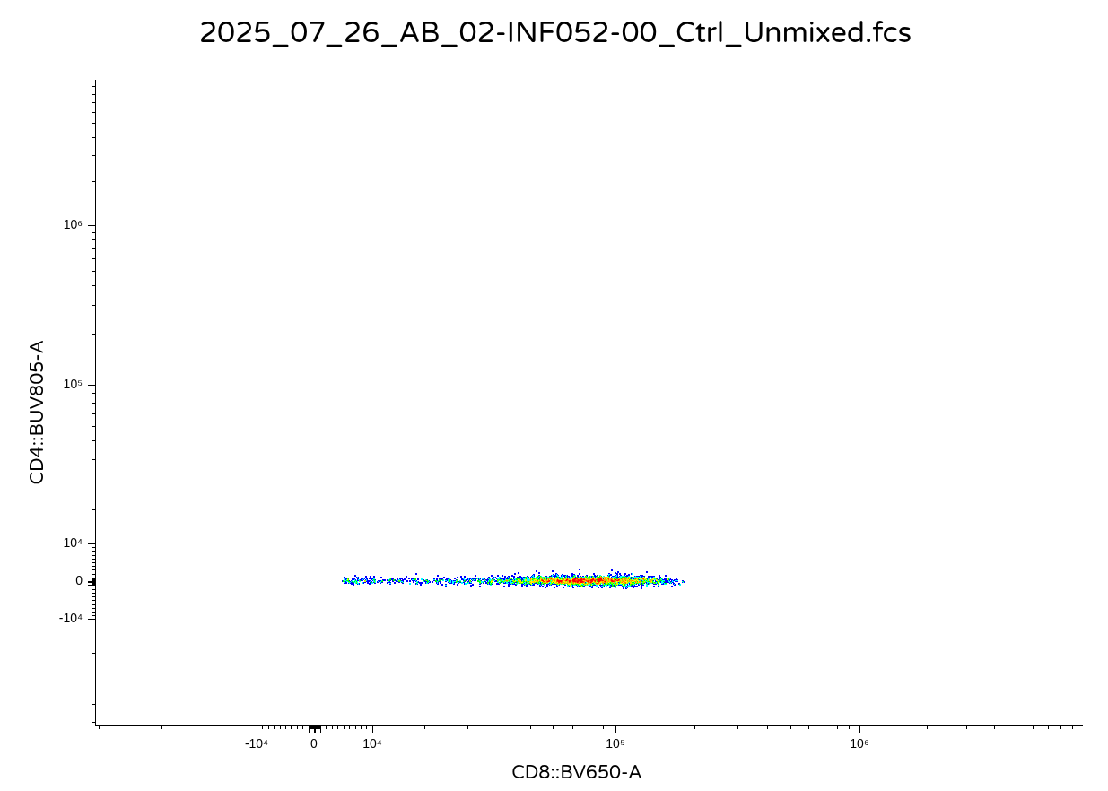
It would likely depend on what you are trying to do. If you plan to remain in R for your data analysis, then keeping these values transformed might make sense for a downstream analysis. Vice versa, if you are exporting out the data as new .fcs files, it is likely you or someone else might want to open them in commercial software. And instead of getting back something that looks like this for a downsampled CD4+ T cell population
![]()
.
You will end up getting back a visual that looks like this
![]()
.
Since the commercial software applies scaling/transformation on top of the existing values (which were previously transformed in R). Consequently, lets go ahead and set ‘inverse.transform’ as Downsampling()’s third argument, but set the default equal to TRUE, since the main use case for today is ability to export out as .fcs files.
#' This function downsamples from a designated gate to our desired number
#' of cells, returning as a new .fcs file
#'
#' @param x A GatingSet object, typically iterated in.
#' @param subset The gate from which to retrieve cell counts from
#' @param inverse.transform Whether to revert values back to their
#' original untransformed values before export as an .fcs file, default
#' is set to TRUE
#'
Downsampling <- function(x, subset, inverse.transform=TRUE){
  EventsInTheGate <- gs_pop_get_data(x, subset,
   inverse.transform=inverse.transform)
  MeasurementData <- exprs(EventsInTheGate[[1]])
  summary(MeasurementData)
}[[1]]
Time SSC-W SSC-H SSC-A
Min. : 19 Min. : 668906 Min. : 99153 Min. : 149656
1st Qu.:223276 1st Qu.: 746226 1st Qu.: 374691 1st Qu.: 481748
Median :446601 Median : 765489 Median : 444238 Median : 567915
Mean :444126 Mean : 771548 Mean : 451345 Mean : 579404
3rd Qu.:664988 3rd Qu.: 787334 3rd Qu.: 514309 3rd Qu.: 657794
Max. :896504 Max. :1333696 Max. :2412543 Max. :3211955
FSC-W FSC-H FSC-A SSC-B-W
Min. :654257 Min. : 775895 Min. : 935556 Min. : 650346
1st Qu.:711727 1st Qu.:1159357 1st Qu.:1396508 1st Qu.: 727882
Median :724892 Median :1305759 Median :1585267 Median : 747608
Mean :725723 Mean :1296808 Mean :1570172 Mean : 754191
3rd Qu.:738849 3rd Qu.:1435574 3rd Qu.:1749781 3rd Qu.: 771752
Max. :821290 Max. :2040353 Max. :2428548 Max. :1430571
SSC-B-H SSC-B-A BUV395-A BUV563-A
Min. : 104214 Min. : 149874 Min. :-2119 Min. : -5749
1st Qu.: 310103 1st Qu.: 388649 1st Qu.: 1871 1st Qu.: 2920
Median : 361253 Median : 453426 Median : 4889 Median : 5982
Mean : 369627 Mean : 464231 Mean : 7093 Mean : 9349
3rd Qu.: 417589 3rd Qu.: 523766 3rd Qu.:10221 3rd Qu.: 11964
Max. :2591438 Max. :3461184 Max. :68245 Max. :221842
BUV615-A BUV661-A BUV737-A BUV805-A
Min. :-10901.65 Min. : -2940.12 Min. :-1613 Min. :-2572.1
1st Qu.: -469.26 1st Qu.: -255.84 1st Qu.: 3319 1st Qu.: 356.7
Median : -46.66 Median : 31.99 Median : 6511 Median :24821.6
Mean : 195.67 Mean : 322.63 Mean : 7355 Mean :19994.0
3rd Qu.: 410.98 3rd Qu.: 333.59 3rd Qu.:10308 3rd Qu.:32942.7
Max. : 27270.46 Max. :144904.06 Max. :38108 Max. :84099.4
Pacific Blue-A BV480-A BV570-A BV605-A
Min. :-4104.3 Min. : -2878.1 Min. :-2457.97 Min. : -3565
1st Qu.: 202.4 1st Qu.: -151.0 1st Qu.: -436.79 1st Qu.: 11084
Median : 472.4 Median : 205.8 Median : 41.05 Median : 22096
Mean : 477.3 Mean : 1086.5 Mean : 98.10 Mean : 28787
3rd Qu.: 747.9 3rd Qu.: 604.0 3rd Qu.: 507.01 3rd Qu.: 39297
Max. :22304.6 Max. :2885917.8 Max. :55880.32 Max. :198982
BV650-A BV711-A BV750-A BV786-A
Min. : -4697.76 Min. :-4487.03 Min. :-1888.3 Min. :-3528.03
1st Qu.: -72.62 1st Qu.: -513.96 1st Qu.: 243.6 1st Qu.: -566.90
Median : 374.00 Median : 48.01 Median : 747.2 Median : 51.42
Mean : 21458.82 Mean : 121.51 Mean : 859.3 Mean : 136.27
3rd Qu.: 33262.86 3rd Qu.: 560.78 3rd Qu.: 1310.0 3rd Qu.: 694.48
Max. :217840.59 Max. :38725.14 Max. :10592.2 Max. :47909.14
Alexa Fluor 488-A Spark Blue 550-A Spark Blue 574-A RB613-A
Min. :-9797.46 Min. :12911 Min. : 5467 Min. : -4391.1
1st Qu.: 85.32 1st Qu.:23719 1st Qu.: 9729 1st Qu.: -308.6
Median : 386.85 Median :29626 Median :11846 Median : 285.4
Mean : 500.52 Mean :30880 Mean :12133 Mean : 1942.0
3rd Qu.: 745.77 3rd Qu.:36515 3rd Qu.:14102 3rd Qu.: 1091.1
Max. :17081.65 Max. :66305 Max. :27834 Max. :117274.7
RB705-A RB780-A PE-A PE-Dazzle594-A
Min. : -1719 Min. :-2673.24 Min. :-16555.3 Min. :-2327.7
1st Qu.: 14886 1st Qu.: -315.76 1st Qu.: 700.8 1st Qu.: 154.9
Median : 39858 Median : 99.64 Median : 1580.2 Median : 558.2
Mean : 41906 Mean : 138.78 Mean : 1834.2 Mean : 598.7
3rd Qu.: 62916 3rd Qu.: 533.22 3rd Qu.: 2651.6 3rd Qu.: 996.7
Max. :253578 Max. :42321.43 Max. : 20731.3 Max. : 7537.0
PE-Cy5-A PE-Fire 700-A PE-Fire 744-A PE-Vio770-A
Min. :-1413.2 Min. :-1175 Min. :-2589.60 Min. : -1751.47
1st Qu.: 75.8 1st Qu.: 2609 1st Qu.: -247.61 1st Qu.: 34.38
Median : 393.3 Median : 4422 Median : 86.36 Median : 428.07
Mean : 1293.7 Mean : 5095 Mean : 783.94 Mean : 840.14
3rd Qu.: 1141.1 3rd Qu.: 6834 3rd Qu.: 430.02 3rd Qu.: 913.96
Max. :53463.8 Max. :33774 Max. :71529.88 Max. :426086.69
APC-A Alexa Fluor 647-A APC-R700-A Zombie NIR-A
Min. : -6016.86 Min. :-2979.07 Min. :-2228.60 Min. :-1025.9
1st Qu.: -19.34 1st Qu.: -375.51 1st Qu.: -78.22 1st Qu.: 401.4
Median : 410.61 Median : 52.78 Median : 251.52 Median : 805.5
Mean : 604.23 Mean : 35.54 Mean : 285.59 Mean : 851.8
3rd Qu.: 859.59 3rd Qu.: 460.81 3rd Qu.: 595.73 3rd Qu.: 1253.9
Max. :101602.37 Max. : 7755.29 Max. : 9522.48 Max. : 3148.6
APC-Fire 750-A APC-Fire 810-A AF-A
Min. :-1696 Min. :-1188 Min. :-12192
1st Qu.:10091 1st Qu.: 5535 1st Qu.: 3386
Median :13641 Median : 9474 Median : 4267
Mean :13841 Mean : 9351 Mean : 4166
3rd Qu.:17338 3rd Qu.:12925 3rd Qu.: 5029
Max. :44324 Max. :34475 Max. : 11486 Subsetting
.
Now that Downsampling() is returning the correct underlying MFI measurement data for our gate of interest, let’s start setting up the code to take the existing number of rows and downsample them to match a desired number of cells. A useful place to pick up at is confirming what type of object we are working with by adding class() back in on our last named object inside the function.
#' This function downsamples from a designated gate to our desired number
#' of cells, returning as a new .fcs file
#'
#' @param x A GatingSet object, typically iterated in.
#' @param subset The gate from which to retrieve cell counts from
#' @param inverse.transform Whether to revert values back to their
#' original untransformed values before export as an .fcs file, default
#' is set to TRUE
#'
Downsampling <- function(x, subset, inverse.transform=TRUE){
  EventsInTheGate <- gs_pop_get_data(x, subset,
   inverse.transform=inverse.transform)
  MeasurementData <- exprs(EventsInTheGate[[1]])
  class(MeasurementData)
}.
While matrices are also rectangular in shape, they are often not as easy to manipulate compared to “data.frame” or “tibble” objects. Let’s go ahead and convert our matrix into a data.frame using as.data.frame().
#' This function downsamples from a designated gate to our desired number
#' of cells, returning as a new .fcs file
#'
#' @param x A GatingSet object, typically iterated in.
#' @param subset The gate from which to retrieve cell counts from
#' @param inverse.transform Whether to revert values back to their
#' original untransformed values before export as an .fcs file, default
#' is set to TRUE
#'
Downsampling <- function(x, subset, inverse.transform=TRUE){
  EventsInTheGate <- gs_pop_get_data(x, subset,
   inverse.transform=inverse.transform)
  MeasurementData <- exprs(EventsInTheGate[[1]])
  MeasurementDataFramed <- as.data.frame(MeasurementData, check.names = FALSE)
  class(MeasurementDataFramed)
}.
Having a ‘data.frame’ object returned, lets switch out our current class() readout for nrow(), so that we can see how many cells we are working with before setting up the downsample code.
#' This function downsamples from a designated gate to our desired number
#' of cells, returning as a new .fcs file
#'
#' @param x A GatingSet object, typically iterated in.
#' @param subset The gate from which to retrieve cell counts from
#' @param inverse.transform Whether to revert values back to their
#' original untransformed values before export as an .fcs file, default
#' is set to TRUE
#'
Downsampling <- function(x, subset, inverse.transform=TRUE){
  EventsInTheGate <- gs_pop_get_data(x, subset,
   inverse.transform=inverse.transform)
  MeasurementData <- exprs(EventsInTheGate[[1]])
  MeasurementDataFramed <- as.data.frame(MeasurementData, check.names = FALSE)
  nrow(MeasurementDataFramed)
}.
When we downsample from our existing data.frame, we would want to be able to retrieve out a specific number of cells (corresponding to individual rows) for a given specimen. These would ideally be selected randomly (and without replacement) so the return we get back would ideally be representative of what we would had seen for the original specimen.
.
Fortunately, dplyr’s slice_sample() function is set up to do this for us, so we can set up its line of code within Downsampling(). In this case, we are passing slice_sample() our data.frame, an outside argument (DownsampleCount), and setting the replace argument to FALSE to accomplish this.
#' This function downsamples from a designated gate to our desired number
#' of cells, returning as a new .fcs file
#'
#' @param x A GatingSet object, typically iterated in.
#' @param subset The gate from which to retrieve cell counts from
#' @param inverse.transform Whether to revert values back to their
#' original untransformed values before export as an .fcs file, default
#' is set to TRUE
#' @param DownsampleCount The desired number of cells to downsample from
#' each gated population.
#'
Downsampling <- function(x, subset, inverse.transform=TRUE, DownsampleCount){
  EventsInTheGate <- gs_pop_get_data(x, subset,
   inverse.transform=inverse.transform)
  MeasurementData <- exprs(EventsInTheGate[[1]])
  MeasurementDataFramed <- as.data.frame(MeasurementData, check.names = FALSE)

  Downsampled_DataFrame <- slice_sample(MeasurementDataFramed, n = DownsampleCount, replace = FALSE)

  nrow(Downsampled_DataFrame)
}.
Seing as we have now downsampled to our target number of cells, let’s switch from using nrow() for return(), so that our returned object is the actual MFI values. To keep things orderly for the website, lets temporarily switch our “DownsampleCount” argument to 10.
#' This function downsamples from a designated gate to our desired number
#' of cells, returning as a new .fcs file
#'
#' @param x A GatingSet object, typically iterated in.
#' @param subset The gate from which to retrieve cell counts from
#' @param inverse.transform Whether to revert values back to their
#' original untransformed values before export as an .fcs file, default
#' is set to TRUE
#' @param DownsampleCount The desired number of cells to downsample from
#' each gated population.
#'
Downsampling <- function(x, subset, inverse.transform=TRUE, DownsampleCount){
  EventsInTheGate <- gs_pop_get_data(x, subset,
   inverse.transform=inverse.transform)
  MeasurementData <- exprs(EventsInTheGate[[1]])
  MeasurementDataFramed <- as.data.frame(MeasurementData, check.names = FALSE)

  Downsampled_DataFrame <- slice_sample(MeasurementDataFramed, n = DownsampleCount, replace = FALSE)

  return(Downsampled_DataFrame)
}[[1]]
Time SSC-W SSC-H SSC-A FSC-W FSC-H FSC-A SSC-B-W SSC-B-H
1 502671 810947.4 585420 791241.4 736648.9 1432357 1758574 818491.4 455846
2 107802 774748.2 339147 437922.5 704972.8 1076277 1264576 758776.4 336020
3 79363 867108.6 431967 624270.5 761632.4 1245655 1581218 841332.8 369241
4 651876 769512.9 497833 638481.6 717618.9 1483911 1774804 745061.3 420928
5 789203 756252.5 388350 489484.4 732302.8 1312617 1602055 733465.5 304457
6 174621 776738.6 443186 573732.8 748718.3 1234603 1540616 768930.8 341485
7 671303 825211.1 337610 464332.5 731789.4 1148257 1400470 793923.9 299127
8 433778 820257.8 592876 810518.6 739588.2 1556729 1918897 811156.6 445763
9 743333 738545.8 423559 521362.8 720530.9 1453384 1745347 697088.9 404135
10 434708 795589.2 340483 451474.3 696226.6 966888 1121955 773525.2 344484
SSC-B-A BUV395-A BUV563-A BUV615-A BUV661-A BUV737-A BUV805-A
1 621843.4 21972.902 2188.6704 624.8232 -155.68594 7069.8770 37229.40625
2 424940.1 6902.792 4909.2715 584.0777 -202.48682 18306.9805 18575.68359
3 517757.6 17131.188 -130.0509 368.3021 -351.45709 10891.0957 35040.84766
4 522695.3 15788.669 2758.4219 193.5819 48.08908 22837.5566 30554.75195
5 372181.2 4195.748 6698.9653 -460.8180 406.74994 16585.8242 32899.69141
6 437630.5 1487.736 3416.6809 -213.8528 -631.26428 5465.8828 443.17099
7 395806.8 9641.060 5062.9741 108.8025 935.82568 -107.3858 349.27551
8 602639.4 22058.365 8274.8623 259.4336 -60.91823 10261.2422 33794.21875
9 469530.0 3792.171 10656.9941 460.6159 325.29398 6843.4243 32725.49414
10 444111.8 1168.579 2649.0020 348.0507 735.49542 1921.4902 -96.85047
Pacific Blue-A BV480-A BV570-A BV605-A BV650-A BV711-A
1 715.30237 323.25571 -154.2919 15582.079 -207.7512 767.8467
2 1136.98999 546.73181 -431.7211 21962.172 364.6723 -833.1782
3 883.72180 -79.13465 -735.2286 38418.547 743.0826 233.4286
4 818.93787 -91.67809 -1119.2245 28263.871 -216.7017 539.3878
5 148.79161 588.05951 721.0452 5799.080 2940.4390 423.9257
6 27.98592 -30.57130 -359.9844 25950.520 87261.5469 -387.0959
7 -123.21954 340.53842 -806.5032 114532.906 3630.9497 909.4780
8 529.40564 -284.06070 639.9856 27460.965 413.6661 399.8089
9 860.13574 -237.88678 506.7387 8970.224 255.6832 21742.9629
10 -699.15704 403.45013 -483.1808 51168.426 58291.5547 -2254.2266
BV750-A BV786-A Alexa Fluor 488-A Spark Blue 550-A Spark Blue 574-A
1 359.00259 1123.73718 91.29433 49523.39 15927.435
2 1389.71265 -1221.97046 987.61310 36282.06 11550.562
3 -62.47601 1422.07471 79.76239 26224.78 15994.604
4 1130.16614 78.54124 438.73447 56874.01 19287.676
5 640.13422 1084.57483 656.59430 30975.80 15378.824
6 1462.78589 -1112.61646 203.90477 29060.37 11196.728
7 48.82246 -121.03413 -224.74390 23077.88 13336.523
8 1220.81934 1320.56152 172.66922 40188.05 9733.442
9 882.80988 977.87781 266.61353 46069.70 9560.861
10 664.15710 -1002.74219 603.81238 21258.35 8731.649
RB613-A RB705-A RB780-A PE-A PE-Dazzle594-A PE-Cy5-A
1 1662.30737 42672.1797 726.5042 4320.0215 293.12741 58.25873
2 1245.71790 54481.3086 279.1711 2889.6343 62.36621 351.36603
3 -339.78564 44564.0703 684.2172 3947.5566 679.33643 190.47656
4 24.54696 72877.3828 657.5319 3417.7234 595.63403 405.04141
5 -416.71390 16852.2910 -603.0715 1513.8683 526.15796 27.49659
6 -688.71545 22097.6738 -455.0402 1085.1472 1368.88879 712.35248
7 9803.41113 -668.3911 -578.8039 62.4234 2237.78442 11583.69238
8 1717.30457 49737.0391 253.6262 2151.6863 138.71523 -85.70993
9 -143.83929 72717.6875 157.7633 1357.9452 655.72406 -616.90460
10 -1126.78662 37678.8906 -434.8350 335.2139 1906.47705 923.92902
PE-Fire 700-A PE-Fire 744-A PE-Vio770-A APC-A Alexa Fluor 647-A
1 8425.429 464.3199 523.2064 757.0491 -154.96271
2 2853.507 194.0843 -430.1349 272.2778 700.98004
3 3590.610 473.4965 7505.5767 126.1787 743.00427
4 4370.683 207.7872 -105.8322 224.2291 80.90195
5 3427.721 442.9737 -528.5533 -116.0480 204.87645
6 4438.309 312.6708 -206.8598 1659.1212 -1035.33362
7 6494.311 384.4048 1157.6638 429.9446 -690.63245
8 5019.328 210.4117 1006.2581 1221.3728 -522.12854
9 6676.723 -1493.1066 1478.3123 1094.7699 -626.08435
10 3185.009 -149.9396 176.1599 -732.0947 463.54037
APC-R700-A Zombie NIR-A APC-Fire 750-A APC-Fire 810-A AF-A
1 376.81033 820.2836 8220.297 20194.4355 5654.606
2 -221.99600 645.4626 22709.666 17305.4844 2938.834
3 1114.29773 1161.5551 16747.631 11338.5381 5090.667
4 -199.94847 1195.5715 13502.367 14173.4688 4891.951
5 -214.76094 467.7580 16075.643 9952.6631 3189.057
6 320.16544 802.9936 16373.131 10179.3428 4613.332
7 136.07945 874.1859 21510.742 867.7909 4029.650
8 64.61411 1689.3375 11474.636 12826.6689 6217.546
9 47.24212 157.5377 12675.298 6078.4941 4144.740
10 794.40991 972.1733 16552.545 5017.1255 2469.000Alternate Scenario 1
.
All-in-all, our Downsampling() function appears to be in working order. Before moving on to figuring how to convert the data.frame into an .fcs, lets consider a couple things.
.
As we saw, for our dataset, the counts were fairly similar across the board for our ‘Tcells’ gate.
.
But what would happen in a scenario where we provided a downsample count that was greater than the number of cells present in the specimen? Would that work? Or would we get back an error?
.
Lets check with the CD8+ gate, using a count of 2500 (which would not be enough for INF179). Lets also switch back our function readout within the function to nrow() for an easier visual summary check.
#' This function downsamples from a designated gate to our desired number
#' of cells, returning as a new .fcs file
#'
#' @param x A GatingSet object, typically iterated in.
#' @param subset The gate from which to retrieve cell counts from
#' @param inverse.transform Whether to revert values back to their
#' original untransformed values before export as an .fcs file, default
#' is set to TRUE
#' @param DownsampleCount The desired number of cells to downsample from
#' each gated population.
#'
Downsampling <- function(x, subset, inverse.transform=TRUE, DownsampleCount){
  EventsInTheGate <- gs_pop_get_data(x, subset,
   inverse.transform=inverse.transform)
  MeasurementData <- exprs(EventsInTheGate[[1]])
  MeasurementDataFramed <- as.data.frame(MeasurementData, check.names = FALSE)

  Downsampled_DataFrame <- slice_sample(MeasurementDataFramed, n = DownsampleCount, replace = FALSE)

  nrow(Downsampled_DataFrame)
}.
Based on the returns, it appears the default behavior for slice_sample() in this scenario where not enough cells are present is just to return all cells that are currently present. Which is good, so one potential worry off our list.
Alternate Scenario 2
.
Alternatively, what if we wanted to retrieve a certain percentage of cells from within a gate for each individual specimen, rather than a fixed count?
.
While we could write this as an entirely separate function, the smarter way (reusing existing code) would be to set up a conditional.
.
One way to implement this using our existing arguments would be, if our ‘DownsampleCount’ argument is less than 1, this would correspond to the desired downsampling proportion that we would to subsample for the respective gated cell population.
.
So in practice, we would modify the function as follows, and update the documentation, as it is not an immediately obvious practice.
#' This function downsamples from a designated gate to our desired number
#' of cells, returning as a new .fcs file
#'
#' @param x A GatingSet object, typically iterated in.
#' @param subset The gate from which to retrieve cell counts from
#' @param inverse.transform Whether to revert values back to their
#' original untransformed values before export as an .fcs file, default
#' is set to TRUE
#' @param DownsampleCount The desired number of cells to downsample from
#' each gated population. If value is less than 1, subsets out the
#' equivalent proportion from that specimen
#'
Downsampling <- function(x, subset, inverse.transform=TRUE, DownsampleCount){
  EventsInTheGate <- gs_pop_get_data(x, subset,
   inverse.transform=inverse.transform)
  MeasurementData <- exprs(EventsInTheGate[[1]])
  MeasurementDataFramed <- as.data.frame(MeasurementData, check.names = FALSE)

  if (DownsampleCount < 1) {
      Count <- nrow(EventsInTheGate) # Original Count
      Count <- as.numeric(Count) #Sanity Check on Value Type
      Count <- Count*DownsampleCount # Target Cells
      Count <- round(Count, 0)
      DownsampleCount <- Count # Over-writting DownsampleCount used for downsampling
    }


  Downsampled_DataFrame <- slice_sample(MeasurementDataFramed, n = DownsampleCount, replace = FALSE)

  nrow(Downsampled_DataFrame)
}.
And with that, the beating heart of our Downsampling function has now been properly set up.
returnType
.
We should probably start figuring out what object format we want our Downsampling() function to be returning.
.
Having generated a subsetted-exprs-matrix, we could reinsert it into the .fcs file, and write it out to a specific folder. This would allow us to access it for subsequent use later on. We would still however need to make a few additional adjustments to the .fcs file metadata, so that we properly document the changes that have been made (so we don’t end up confusing these downsampled files with the original ones).
.
Alternately, after downsampling, we may just want to return out outputs directly to R for continued analysis. In this scenario, we might want back the data as a ‘data.frame’ object (which wouldn’t have any associated metadata) or as a ‘flowFrame’ or ‘cytoframe’ object (which would have corresponding metadata).
.
Let’s start with the main goal, our downsampled output as an .fcs file, and then add conditionals to allow for the return the other two options.
Creating new .fcs files
.
Remembering back to Week 03, .fcs files in R are made up of 3 slots in the S4 object, ‘exprs’ (which we have been manipulating today), ‘parameters’ (containing general fluorophore/marker panel info), and ‘description/keyword’ (all the other metadata).
.
So far, we have not changed anything in terms of the number of columns, so we shouldn’t need to make any changes to parameters (yey!). But we would need to swap out the existing exprs matrix (corresponding to that of the original .fcs file) for our downsampled one. Similarly, good reproducibility practice means we should update the appropiate keywords so that the generated .fcs files are not the originals.
.
Lets continue by converting our ‘data.frame’ object back to the original ‘matrix’ type object, using the as.matrix() function.
#' This function downsamples from a designated gate to our desired number
#' of cells, returning as a new .fcs file
#'
#' @param x A GatingSet object, typically iterated in.
#' @param subset The gate from which to retrieve cell counts from
#' @param inverse.transform Whether to revert values back to their
#' original untransformed values before export as an .fcs file, default
#' is set to TRUE
#' @param DownsampleCount The desired number of cells to downsample from
#' each gated population. If value is less than 1, subsets out the
#' equivalent proportion from that specimen
#'
Downsampling <- function(x, subset, inverse.transform=TRUE, DownsampleCount){
  EventsInTheGate <- gs_pop_get_data(x, subset,
   inverse.transform=inverse.transform)
  MeasurementData <- exprs(EventsInTheGate[[1]])
  MeasurementDataFramed <- as.data.frame(MeasurementData, check.names = FALSE)

  if (DownsampleCount < 1) {
      Count <- nrow(EventsInTheGate) # Original Count
      Count <- as.numeric(Count) #Sanity Check on Value Type
      Count <- Count*DownsampleCount # Target Cells
      Count <- round(Count, 0)
      DownsampleCount <- Count # Over-writting DownsampleCount used for downsampling
    }


  Downsampled_DataFrame <- slice_sample(MeasurementDataFramed, n = DownsampleCount, replace = FALSE)

  DownsampledMatrix <- as.matrix(Downsampled_DataFrame)
  class(DownsampledMatrix)
}.
As mentioned, we will need to break out and copy the pieces from the original .fcs file into the new .fcs. The easiest way to gain access to all this information is to switch over from a cytoframe (working via a pointer) to a flowFrame (loaded into RAM). This will allow us access to the flowCore helper functions (parameters(), exprs(), and keyword()) to access the corresponding slots.
#' This function downsamples from a designated gate to our desired number
#' of cells, returning as a new .fcs file
#'
#' @param x A GatingSet object, typically iterated in.
#' @param subset The gate from which to retrieve cell counts from
#' @param inverse.transform Whether to revert values back to their
#' original untransformed values before export as an .fcs file, default
#' is set to TRUE
#' @param DownsampleCount The desired number of cells to downsample from
#' each gated population. If value is less than 1, subsets out the
#' equivalent proportion from that specimen
#'
Downsampling <- function(x, subset, inverse.transform=TRUE, DownsampleCount){
  EventsInTheGate <- gs_pop_get_data(x, subset,
   inverse.transform=inverse.transform)
  MeasurementData <- exprs(EventsInTheGate[[1]])
  MeasurementDataFramed <- as.data.frame(MeasurementData, check.names = FALSE)

  if (DownsampleCount < 1) {
      Count <- nrow(EventsInTheGate) # Original Count
      Count <- as.numeric(Count) #Sanity Check on Value Type
      Count <- Count*DownsampleCount # Target Cells
      Count <- round(Count, 0)
      DownsampleCount <- Count # Over-writting DownsampleCount used for downsampling
    }

  Downsampled_DataFrame <- slice_sample(MeasurementDataFramed, n = DownsampleCount, replace = FALSE)

  DownsampledMatrix <- as.matrix(Downsampled_DataFrame)

  flowFrame <- EventsInTheGate[[1, returnType = "flowFrame"]]
  OriginalParameters <- parameters(flowFrame)
  OriginalDescription <- keyword(flowFrame)

  return(OriginalParameters)
}.
Seeing as we now have access to the ‘flowFrame’ contents, we can now cobble together our “DownsampledMatrix” (corresponding to the new ‘exprs’ slot) with the contents of the original ‘description’ and ‘parameters’ slots.
.
With all the components gathered, creating a new .fcs file is as simple as handing them off to the new() function.
#' This function downsamples from a designated gate to our desired number
#' of cells, returning as a new .fcs file
#'
#' @param x A GatingSet object, typically iterated in.
#' @param subset The gate from which to retrieve cell counts from
#' @param inverse.transform Whether to revert values back to their
#' original untransformed values before export as an .fcs file, default
#' is set to TRUE
#' @param DownsampleCount The desired number of cells to downsample from
#' each gated population. If value is less than 1, subsets out the
#' equivalent proportion from that specimen
#'
Downsampling <- function(x, subset, inverse.transform=TRUE, DownsampleCount){
  EventsInTheGate <- gs_pop_get_data(x, subset,
   inverse.transform=inverse.transform)
  MeasurementData <- exprs(EventsInTheGate[[1]])
  MeasurementDataFramed <- as.data.frame(MeasurementData, check.names = FALSE)

  if (DownsampleCount < 1) {
      Count <- nrow(EventsInTheGate) # Original Count
      Count <- as.numeric(Count) #Sanity Check on Value Type
      Count <- Count*DownsampleCount # Target Cells
      Count <- round(Count, 0)
      DownsampleCount <- Count # Over-writting DownsampleCount used for downsampling
    }

  Downsampled_DataFrame <- slice_sample(MeasurementDataFramed, n = DownsampleCount, replace = FALSE)

  DownsampledMatrix <- as.matrix(Downsampled_DataFrame)

  flowFrame <- EventsInTheGate[[1, returnType = "flowFrame"]]
  OriginalParameters <- parameters(flowFrame)
  OriginalDescription <- keyword(flowFrame)

  NewFCS <- new("flowFrame", exprs=DownsampledMatrix, parameters=OriginalParameters, description=OriginalDescription)

  return(NewFCS)
}[[1]]
flowFrame object '2025_07_26_AB_02-INF052-00_Ctrl_Unmixed__Tcells.fcs'
with 2473 cells and 43 observables:
name desc range minRange maxRange
$P1 Time NA 896744 0 896744
$P2 SSC-W NA 4194303 0 4194303
$P3 SSC-H NA 4194303 0 4194303
$P4 SSC-A NA 4194303 0 4194303
$P5 FSC-W NA 4194303 0 4194303
... ... ... ... ... ...
$P39 APC-R700-A CD107a 4194275 -111 4194275
$P40 Zombie NIR-A Viability 4194275 -111 4194275
$P41 APC-Fire 750-A CD27 4194275 -111 4194275
$P42 APC-Fire 810-A CCR7 4194275 -111 4194275
$P43 AF-A NA 4194275 -111 4194275
472 keywords are stored in the 'description' slot.
We are now able to get back a standard flowFrame object. Looking at the readout output, we see that it automatically updated to reflect the new number of downsampled cells, while retaining the metadata from the original .fcs file.
Updating keywords
.
Before calling it good, and saving this flowFrame as an .fccs, lets back up a couple lines and update a few important keywords within the ‘description’ slot, so that we can tell our “downsampled in R” .fcs file apart from the original .fcs file.
.
A simpler way of doing this is setting up another argument (which we will designate as ‘addon’), that will append a character value between the specimens corresponding tubename and the ending .fcs. For this particular instrument manufacturer, changing the “GUID” keyword for this .fcs file makes sense (although the equivalent keyword may vary depending on other platforms).
#' This function downsamples from a designated gate to our desired number
#' of cells, returning as a new .fcs file
#'
#' @param x A GatingSet object, typically iterated in.
#' @param subset The gate from which to retrieve cell counts from
#' @param inverse.transform Whether to revert values back to their
#' original untransformed values before export as an .fcs file, default
#' is set to TRUE
#' @param DownsampleCount The desired number of cells to downsample from
#' each gated population. If value is less than 1, subsets out the
#' equivalent proportion from that specimen
#' @param addon An additional character value to add before .fcs in the GUID
#' keyword to tell the downsampled file apart from the original.
#'
Downsampling <- function(x, subset, inverse.transform=TRUE, DownsampleCount,
  addon){
  EventsInTheGate <- gs_pop_get_data(x, subset,
   inverse.transform=inverse.transform)
  MeasurementData <- exprs(EventsInTheGate[[1]])
  MeasurementDataFramed <- as.data.frame(MeasurementData, check.names = FALSE)

  if (DownsampleCount < 1) {
      Count <- nrow(EventsInTheGate) # Original Count
      Count <- as.numeric(Count) #Sanity Check on Value Type
      Count <- Count*DownsampleCount # Target Cells
      Count <- round(Count, 0)
      DownsampleCount <- Count # Over-writting DownsampleCount used for downsampling
    }

  Downsampled_DataFrame <- slice_sample(MeasurementDataFramed, n = DownsampleCount, replace = FALSE)

  DownsampledMatrix <- as.matrix(Downsampled_DataFrame)

  flowFrame <- EventsInTheGate[[1, returnType = "flowFrame"]]
  OriginalParameters <- parameters(flowFrame)
  OriginalDescription <- keyword(flowFrame)

  OriginalName <- OriginalDescription$`GUID`
  UpdatedName <- paste0("_", addon, ".fcs")
  UpdatedGUID <- sub(".fcs", UpdatedName, OriginalName) #Swtiching out .fcs for Updated Name via the sub function
  OriginalDescription$`GUID` <- UpdatedGUID

  NewFCS <- new("flowFrame", exprs=DownsampledMatrix, parameters=OriginalParameters, description=OriginalDescription)

  return(NewFCS)
}[[1]]
flowFrame object '2025_07_26_AB_02-INF052-00_Ctrl_Unmixed__Tcells_CD8.fcs'
with 2473 cells and 43 observables:
name desc range minRange maxRange
$P1 Time NA 896744 0 896744
$P2 SSC-W NA 4194303 0 4194303
$P3 SSC-H NA 4194303 0 4194303
$P4 SSC-A NA 4194303 0 4194303
$P5 FSC-W NA 4194303 0 4194303
... ... ... ... ... ...
$P39 APC-R700-A CD107a 4194275 -111 4194275
$P40 Zombie NIR-A Viability 4194275 -111 4194275
$P41 APC-Fire 750-A CD27 4194275 -111 4194275
$P42 APC-Fire 810-A CCR7 4194275 -111 4194275
$P43 AF-A NA 4194275 -111 4194275
472 keywords are stored in the 'description' slot.
From the readout, we can see that we are now able to distinguish our file from the original based on atleast this single keyword.
Export as .fcs
.
Lets work in how to export the ‘flowFrame’ out as a .fcs file, ideally to a designated storage location. Since our now updated GUID keyword already contains “.fcs” at the end, we don’t need to add anything else to the new file name in order to specify the file type. We will just need to add ‘StorageLocation’ as another Downsampling() argument (updating the documentation accordingly), and then do some adjustments internally to generate a full file.path().
#' This function downsamples from a designated gate to our desired number
#' of cells, returning as a new .fcs file
#'
#' @param x A GatingSet object, typically iterated in.
#' @param subset The gate from which to retrieve cell counts from
#' @param inverse.transform Whether to revert values back to their
#' original untransformed values before export as an .fcs file, default
#' is set to TRUE
#' @param DownsampleCount The desired number of cells to downsample from
#' each gated population. If value is less than 1, subsets out the
#' equivalent proportion from that specimen
#' @param addon An additional character value to add before .fcs in the GUID
#' keyword to tell the downsampled file apart from the original.
#' @param StorageLocation A file.path to the folder you want to store the new downsampled
#' fcs file to.
#'
Downsampling <- function(x, subset, inverse.transform=TRUE, DownsampleCount,
  addon, StorageLocation){
  EventsInTheGate <- gs_pop_get_data(x, subset,
   inverse.transform=inverse.transform)
  MeasurementData <- exprs(EventsInTheGate[[1]])
  MeasurementDataFramed <- as.data.frame(MeasurementData, check.names = FALSE)

  if (DownsampleCount < 1) {
      Count <- nrow(EventsInTheGate) # Original Count
      Count <- as.numeric(Count) #Sanity Check on Value Type
      Count <- Count*DownsampleCount # Target Cells
      Count <- round(Count, 0)
      DownsampleCount <- Count # Over-writting DownsampleCount used for downsampling
    }

  Downsampled_DataFrame <- slice_sample(MeasurementDataFramed, n = DownsampleCount, replace = FALSE)

  DownsampledMatrix <- as.matrix(Downsampled_DataFrame)

  flowFrame <- EventsInTheGate[[1, returnType = "flowFrame"]]
  OriginalParameters <- parameters(flowFrame)
  OriginalDescription <- keyword(flowFrame)

  OriginalName <- OriginalDescription$`GUID`
  UpdatedName <- paste0("_", addon, ".fcs")
  UpdatedGUID <- sub(".fcs", UpdatedName, OriginalName) #Swtiching out .fcs for Updated Name via the sub function
  OriginalDescription$`GUID` <- UpdatedGUID

  NewFCS <- new("flowFrame", exprs=DownsampledMatrix, parameters=OriginalParameters, description=OriginalDescription)

  StoreFCSFileHere <- file.path(StorageLocation, UpdatedGUID)

  return(StoreFCSFileHere)
}.
As we have encountered previously, if no value is provided to an argument, it returns back as an error. Consequently, adding a default option would make sense in this case. We can use the getwd() function to identify the file.path to the current working directory, which will be used as the standin in case we don’t end up specifying a ‘StorageLocation’ file.path.
.
By setting the default argument value for ‘StorageLocation’ equal to NULL (i.e. nothing), we can use an ‘if’ conditional in combination with is.null() to handle this situation when encountered.
#' This function downsamples from a designated gate to our desired number
#' of cells, returning as a new .fcs file
#'
#' @param x A GatingSet object, typically iterated in.
#' @param subset The gate from which to retrieve cell counts from
#' @param inverse.transform Whether to revert values back to their
#' original untransformed values before export as an .fcs file, default
#' is set to TRUE
#' @param DownsampleCount The desired number of cells to downsample from
#' each gated population. If value is less than 1, subsets out the
#' equivalent proportion from that specimen
#' @param addon An additional character value to add before .fcs in the GUID
#' keyword to tell the downsampled file apart from the original.
#' @param StorageLocation A file.path to the folder you want to store the new downsampled
#' fcs file to. Default NULL results in .fcs file being stored in current working directory
#'
#'
Downsampling <- function(x, subset, inverse.transform=TRUE, DownsampleCount,
  addon, StorageLocation=NULL){
  EventsInTheGate <- gs_pop_get_data(x, subset,
   inverse.transform=inverse.transform)
  MeasurementData <- exprs(EventsInTheGate[[1]])
  MeasurementDataFramed <- as.data.frame(MeasurementData, check.names = FALSE)

  if (DownsampleCount < 1) {
      Count <- nrow(EventsInTheGate) # Original Count
      Count <- as.numeric(Count) #Sanity Check on Value Type
      Count <- Count*DownsampleCount # Target Cells
      Count <- round(Count, 0)
      DownsampleCount <- Count # Over-writting DownsampleCount used for downsampling
    }

  Downsampled_DataFrame <- slice_sample(MeasurementDataFramed, n = DownsampleCount, replace = FALSE)

  DownsampledMatrix <- as.matrix(Downsampled_DataFrame)

  flowFrame <- EventsInTheGate[[1, returnType = "flowFrame"]]
  OriginalParameters <- parameters(flowFrame)
  OriginalDescription <- keyword(flowFrame)

  OriginalName <- OriginalDescription$`GUID`
  UpdatedName <- paste0("_", addon, ".fcs")
  UpdatedGUID <- sub(".fcs", UpdatedName, OriginalName) #Swtiching out .fcs for Updated Name via the sub function
  OriginalDescription$`GUID` <- UpdatedGUID

  NewFCS <- new("flowFrame", exprs=DownsampledMatrix, parameters=OriginalParameters, description=OriginalDescription)

  if (is.null(StorageLocation)){StorageLocation <- getwd()}

  StoreFCSFileHere <- file.path(StorageLocation, UpdatedGUID)

  return(StoreFCSFileHere)
}.
Having the full file path and corresponding new name now specified within Downsampling(), we are now ready to write our first new .fcs file. This is accomplished through the flowCore packages write.FCS() function, which we will add in at the end of our function.
#' This function downsamples from a designated gate to our desired number
#' of cells, returning as a new .fcs file
#'
#' @param x A GatingSet object, typically iterated in.
#' @param subset The gate from which to retrieve cell counts from
#' @param inverse.transform Whether to revert values back to their
#' original untransformed values before export as an .fcs file, default
#' is set to TRUE
#' @param DownsampleCount The desired number of cells to downsample from
#' each gated population. If value is less than 1, subsets out the
#' equivalent proportion from that specimen
#' @param addon An additional character value to add before .fcs in the GUID
#' keyword to tell the downsampled file apart from the original.
#' @param StorageLocation A file.path to the folder you want to store the new downsampled
#' fcs file to. Default NULL results in .fcs file being stored in current working directory
#'
#'
Downsampling <- function(x, subset, inverse.transform=TRUE, DownsampleCount,
  addon, StorageLocation=NULL){
  EventsInTheGate <- gs_pop_get_data(x, subset,
   inverse.transform=inverse.transform)
  MeasurementData <- exprs(EventsInTheGate[[1]])
  MeasurementDataFramed <- as.data.frame(MeasurementData, check.names = FALSE)

  if (DownsampleCount < 1) {
      Count <- nrow(EventsInTheGate) # Original Count
      Count <- as.numeric(Count) #Sanity Check on Value Type
      Count <- Count*DownsampleCount # Target Cells
      Count <- round(Count, 0)
      DownsampleCount <- Count # Over-writting DownsampleCount used for downsampling
    }

  Downsampled_DataFrame <- slice_sample(MeasurementDataFramed, n = DownsampleCount, replace = FALSE)

  DownsampledMatrix <- as.matrix(Downsampled_DataFrame)

  flowFrame <- EventsInTheGate[[1, returnType = "flowFrame"]]
  OriginalParameters <- parameters(flowFrame)
  OriginalDescription <- keyword(flowFrame)

  OriginalName <- OriginalDescription$`GUID`
  UpdatedName <- paste0("_", addon, ".fcs")
  UpdatedGUID <- sub(".fcs", UpdatedName, OriginalName) #Swtiching out .fcs for Updated Name via the sub function
  OriginalDescription$`GUID` <- UpdatedGUID

  NewFCS <- new("flowFrame", exprs=DownsampledMatrix, parameters=OriginalParameters, description=OriginalDescription)

  if (is.null(StorageLocation)){StorageLocation <- getwd()}

  StoreFCSFileHere <- file.path(StorageLocation, UpdatedGUID)
  write.FCS(NewFCS, filename = StoreFCSFileHere, delimiter="#")

  return(StoreFCSFileHere)
}
.
We have now returned our .fcs file. For a quick sanity check (and so that my collaborators don’t track me down later in the day reporting odd scaling issue), lets double check it opens correctly using Floreada.io or other flow software.
Alternate Export Options
.
Now that we can export as a ‘.fcs’ file, lets wrap up by providing the option to instead return either the ‘data.frame’ or the ‘flowFrame’ object (if we wished to continue working with them in R). We can do set up within Downsampling() a new argument (returnType) and a couple branching conditional statements with ‘if’ and ‘ifelse’ to designate the different outcomes for different provided argument values.
#' This function downsamples from a designated gate to our desired number
#' of cells, returning as a new .fcs file
#'
#' @param x A GatingSet object, typically iterated in.
#' @param subset The gate from which to retrieve cell counts from
#' @param inverse.transform Whether to revert values back to their
#' original untransformed values before export as an .fcs file, default
#' is set to TRUE
#' @param DownsampleCount The desired number of cells to downsample from
#' each gated population. If value is less than 1, subsets out the
#' equivalent proportion from that specimen
#' @param addon An additional character value to add before .fcs in the GUID
#' keyword to tell the downsampled file apart from the original.
#' @param StorageLocation A file.path to the folder you want to store the new downsampled
#' fcs file to. Default NULL results in .fcs file being stored in current working directory
#' @param returnType Whether to return as a "fcs" file (default), or "flowFrame" or "data.frame"
#'
#'
Downsampling <- function(x, subset, inverse.transform=TRUE, DownsampleCount,
  addon, StorageLocation=NULL, returnType="fcs"){
  EventsInTheGate <- gs_pop_get_data(x, subset,
   inverse.transform=inverse.transform)
  MeasurementData <- exprs(EventsInTheGate[[1]])
  MeasurementDataFramed <- as.data.frame(MeasurementData, check.names = FALSE)

  if (DownsampleCount < 1) {
      Count <- nrow(EventsInTheGate) # Original Count
      Count <- as.numeric(Count) #Sanity Check on Value Type
      Count <- Count*DownsampleCount # Target Cells
      Count <- round(Count, 0)
      DownsampleCount <- Count # Over-writting DownsampleCount used for downsampling
    }

  Downsampled_DataFrame <- slice_sample(MeasurementDataFramed, n = DownsampleCount, replace = FALSE)

  DownsampledMatrix <- as.matrix(Downsampled_DataFrame)

  flowFrame <- EventsInTheGate[[1, returnType = "flowFrame"]]
  OriginalParameters <- parameters(flowFrame)
  OriginalDescription <- keyword(flowFrame)

  OriginalName <- OriginalDescription$`GUID`
  UpdatedName <- paste0("_", addon, ".fcs")
  UpdatedGUID <- sub(".fcs", UpdatedName, OriginalName) #Swtiching out .fcs for Updated Name via the sub function
  OriginalDescription$`GUID` <- UpdatedGUID

  NewFCS <- new("flowFrame", exprs=DownsampledMatrix, parameters=OriginalParameters, description=OriginalDescription)

  if (is.null(StorageLocation)){StorageLocation <- getwd()}

  StoreFCSFileHere <- file.path(StorageLocation, UpdatedGUID)


  if (returnType == "fcs"){
    write.FCS(NewFCS, filename = StoreFCSFileHere, delimiter="#") # Write out .fcs file
  } else if (returnType == "data.frame"){
    return(Downsampled_DataFrame) #Return data.frame without metadata
  } else {
    return(NewFCS) #All other criterias return a flowFrame with metadata
    }

}
Data <- map(.x=SFC_GatingSet[1], subset="CD8+", .f=Downsampling, DownsampleCount=2500, addon="CD8",
returnType="data.frame")
head(Data[[1]], 3) Time SSC-W SSC-H SSC-A FSC-W FSC-H FSC-A SSC-B-W SSC-B-H
1 465570 765146.9 466353 594714.2 770175.8 1456597 1869726 752907.6 373349
2 444495 774441.3 285712 368778.6 696686.0 1233000 1431690 737545.1 273244
3 521722 785098.4 425786 557139.8 719176.5 1240402 1486780 773852.5 410139
SSC-B-A BUV395-A BUV563-A BUV615-A BUV661-A BUV737-A BUV805-A
1 468495.5 66.76678 13098.539 -112.9783 344.9401 1344.863 -426.4513
2 335883.0 1274.67078 2405.598 -415.4337 -421.6886 5404.412 -570.6855
3 528978.5 349.28171 16117.677 613.0233 529.5594 6221.521 384.7617
Pacific Blue-A BV480-A BV570-A BV605-A BV650-A BV711-A BV750-A
1 565.3184 7755.0181 150.38908 2942.396 15847.86 25.76186 959.9550
2 -1051.0872 560.8405 36.93896 53214.539 86881.62 -505.50708 743.0158
3 -364.2599 783.6228 218.62964 51365.730 52253.37 -197.31549 1123.8638
BV786-A Alexa Fluor 488-A Spark Blue 550-A Spark Blue 574-A RB613-A
1 -260.9827 808.5419 23525.88 9126.426 37005.57422
2 -223.3768 80.3253 20946.10 10018.960 28.51259
3 -305.0150 672.6376 16410.83 11344.572 1044.24463
RB705-A RB780-A PE-A PE-Dazzle594-A PE-Cy5-A PE-Fire 700-A
1 291.4547 -575.4986 1130.14404 173.4328 1252.3345 -911.9573
2 17797.5801 448.4373 -76.11315 783.8643 883.3913 2714.6113
3 6997.2485 626.7309 2155.92676 424.8021 3649.7964 2472.1133
PE-Fire 744-A PE-Vio770-A APC-A Alexa Fluor 647-A APC-R700-A Zombie NIR-A
1 467.7792 414.2708 -458.8768 -122.4269 533.4082 776.2895
2 188.5845 -480.7317 1883.3727 -1225.1925 272.7380 436.4146
3 -333.9474 -208.5314 1414.6920 -1379.3351 1074.5509 142.3087
APC-Fire 750-A APC-Fire 810-A AF-A
1 2902.586 499.9916 6496.290
2 11683.459 5054.7905 1931.103
3 17538.646 6291.4204 3269.152.
And there we go, Downsampling() now has the functionality to return objects in different formats, depending on what our use case may be.
Dependencies
.
One important thing before proceeding, Downsampling currently works because we called library() on all the packages needed to run the various functions we were using inside of it. If we were to close Positron and reopen, if we forgot to run one of these libraries (let’s say dplyr), we would get the following style error
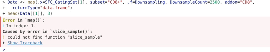
.
Since dplyr is not attached to our local environment, when slice_sample() is encountered within the function, and not defined elsewhere, we get an error returned. While we could remember to load all our various R packages at the start to avoid this issue, this opens another can of worms, as many R packages have functions with identical names, which results in the last package called masking those with identical names before it. This can often cause functions to fail, so less than ideal.
.
There are two ways around this. Later on in the course, we will see how to use the @importFrom tag within a Roxygen2 skeleton, alongside the devtools package load_all() function to specify function-level dependencies from the get-go. However, since a couple additional setup steps are needed, for now, we will default to updating our functions to use the “packageName :: function name” option, with the ‘::’ telling R to use the function from that package regardless if it is currently attached to the local environment or not.
.
In our case, I will go ahead and add the @importFrom tags (syntax is package name, followed by functions being imported from it) within the roxygen skeleton, and then within the function do the equivalent second option using ‘::’
#' This function downsamples from a designated gate to our desired number
#' of cells, returning as a new .fcs file
#'
#' @param x A GatingSet object, typically iterated in.
#' @param subset The gate from which to retrieve cell counts from
#' @param inverse.transform Whether to revert values back to their
#' original untransformed values before export as an .fcs file, default
#' is set to TRUE
#' @param DownsampleCount The desired number of cells to downsample from
#' each gated population. If value is less than 1, subsets out the
#' equivalent proportion from that specimen
#' @param addon An additional character value to add before .fcs in the GUID
#' keyword to tell the downsampled file apart from the original.
#' @param StorageLocation A file.path to the folder you want to store the new downsampled
#' fcs file to. Default NULL results in .fcs file being stored in current working directory
#' @param returnType Whether to return as a "fcs" file (default), or "flowFrame" or "data.frame"
#'
#' @importFrom flowWorkspace gs_pop_get_data
#' @importFrom flowCore parameters keyword write.FCS
#' @importFrom Biobase exprs
#' @importFrom dplyr slice_sample
#'
#'
Downsampling <- function(x, subset, inverse.transform=TRUE, DownsampleCount,
  addon, StorageLocation=NULL, returnType="fcs"){
  EventsInTheGate <- flowWorkspace::gs_pop_get_data(x, subset,
   inverse.transform=inverse.transform)
  MeasurementData <- Biobase::exprs(EventsInTheGate[[1]])
  MeasurementDataFramed <- as.data.frame(MeasurementData, check.names = FALSE)

  if (DownsampleCount < 1) {
      Count <- nrow(EventsInTheGate) # Original Count
      Count <- as.numeric(Count) #Sanity Check on Value Type
      Count <- Count*DownsampleCount # Target Cells
      Count <- round(Count, 0)
      DownsampleCount <- Count # Over-writting DownsampleCount used for downsampling
    }

  Downsampled_DataFrame <- dplyr::slice_sample(MeasurementDataFramed, n = DownsampleCount, replace = FALSE)

  DownsampledMatrix <- as.matrix(Downsampled_DataFrame)

  flowFrame <- EventsInTheGate[[1, returnType = "flowFrame"]]
  OriginalParameters <- flowCore::parameters(flowFrame)
  OriginalDescription <- flowCore::keyword(flowFrame)

  OriginalName <- OriginalDescription$`GUID`
  UpdatedName <- paste0("_", addon, ".fcs")
  UpdatedGUID <- sub(".fcs", UpdatedName, OriginalName) #Swtiching out .fcs for Updated Name via the sub function
  OriginalDescription$`GUID` <- UpdatedGUID

  NewFCS <- new("flowFrame", exprs=DownsampledMatrix, parameters=OriginalParameters, description=OriginalDescription)

  if (is.null(StorageLocation)){StorageLocation <- getwd()}

  StoreFCSFileHere <- file.path(StorageLocation, UpdatedGUID)

  if (returnType == "fcs"){
    flowCore::write.FCS(NewFCS, filename = StoreFCSFileHere, delimiter="#") # Write out .fcs file
  } else if (returnType == "data.frame"){
    return(Downsampled_DataFrame) #Return data.frame without metadata
  } else {
    return(NewFCS) #All other criterias return a flowFrame with metadata
    }

}purrr::map(.x=SFC_GatingSet[1], subset="CD8+", .f=Downsampling, DownsampleCount=2500, addon="CD8",
returnType="flowFrame")[[1]]
flowFrame object '2025_07_26_AB_02-INF052-00_Ctrl_Unmixed__Tcells_CD8.fcs'
with 2473 cells and 43 observables:
name desc range minRange maxRange
$P1 Time NA 896744 0 896744
$P2 SSC-W NA 4194303 0 4194303
$P3 SSC-H NA 4194303 0 4194303
$P4 SSC-A NA 4194303 0 4194303
$P5 FSC-W NA 4194303 0 4194303
... ... ... ... ... ...
$P39 APC-R700-A CD107a 4194275 -111 4194275
$P40 Zombie NIR-A Viability 4194275 -111 4194275
$P41 APC-Fire 750-A CD27 4194275 -111 4194275
$P42 APC-Fire 810-A CCR7 4194275 -111 4194275
$P43 AF-A NA 4194275 -111 4194275
472 keywords are stored in the 'description' slot.
Now, with the flowWorkspace, flowCore, Biobase and dplyr dependencies specied within the function, Downsample runs without issues regardless of whether the packages are attached to our local environment.
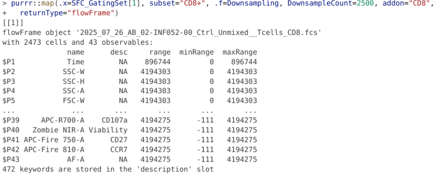
At last
.
We can now remove the indexing ([1]) from SFC_GatingSet that we used throughout the building process, and proceed to downsample our entire GatingSet based on our parameters of interests.
.
For example, returning 2500 CD4+ T cells as .fcs files (to my desktop file.path)
.
Or 10% of all T cells (to my desktop file.path)
Export
.
Now that we have fully assembled Downsampling(), there is actually another useful use case when it comes to its ability to export out as fully-compatible .fcs files. If instead of providing a downsample number, we provided an implausibly high number (lets say 10,000,000) we would basically directly export out the entire gated cell population of interest as its own .fcs file.
.
This can be quite useful, as you can set up your cleanup gates and major cell population gates (double checking to make sure they are applied correctly), and then export out your actual cell populations of interest as smaller .fcs files for future analysis. That way, if you are implementing hybrid workflows with large spectral flow cytometry files relying on commercial software (similar to the Flow-Jo/CytoML example from Week 05), you do not crash your RAM just trying to open the workspace.
Concatenate
Nested Functions
.
So far, we have continued the process of learning how to write our own functions to carry out useful tasks, culminating in creating our Downsampling function. While downsampling itself can be useful in certain situations, it is often used as part of a workflow where the downsampled outputs are combined together into a single .fcs file (concatenation) for use in unsupervised workflows (like dimensionality visualization).
.
Unlike Downsampling(), which works within an individual .fcs files at a time, if we were to build out a Concatenate() function, we would need to first retrieve the downsampled returns from every .fcs file via iteration, then combine them together, before outputting them as a new .fcs file.
.
The tricky part is that in practice, often when we Concatenate, we want to add in keywords to be able to tell the cells coming from the individual contributors of the concatenated file apart after the fact. For .fcs files, these keywords end up becoming additional columns in the ‘exprs’ matrix, which causes the need to not only modify exprs, but also parameters and description slots rather extensively before we can create the new .fcs file.
.
However, I promised to not drown you in your first forray to the deep-end of the pool, so there will be no more function building in this session. I will provide the out code for Concatenate() and its various nested helper functions below, and instead focus on how to use it for actual implementation within our workflows for the rest of the time we have left.
.
If, however, you are not burnt out on function building and want to optionally read through the equivalent Concatenate walk-through, follow the link here.
Concatenate Code
.
Briefly as far as explainers go, Concatenate needs to iterate through various .fcs files to retrieve the Downsampling outputs, as well as extract corresponding metadata for each iterated .fcs file. These get added in as new columns, with the cascading changes ending up applied to ‘exprs’, ‘parameters’, and ‘keyword’ slots, before being outputted as our return object type of choice. Because of all these moving parts, Concatenate is an example of a nested function, with several smaller helper functions that are called to help carry out the individual tasks.
.
To see the Concatenate and associated helper functions, click the code-show arrow below. To skip the code and start using them, run the “Run Cell” option to get them to appear correctly in your local environment.
Code
#' Concatenate Internal
#'
#' @param x TBD
#' @param y TBD
#' @param metadata TBD
#'
#' @importFrom dplyr filter bind_cols
#'
KeywordAppend <- function(x, y, metadata) {
  df <- y
  rownames(metadata) <- NULL
  AddThisRow <- metadata |> filter(name %in% x)
  ExpandedData <- bind_cols(df, AddThisRow)
  return(ExpandedData)
}

#' Concatenate Internal
#'
#' @param DictionaryList TBD
#' @param data TBD
#'
#' @importFrom dplyr left_join select rename
#' @importFrom tidyselect all_of
#' @importFrom rlang sym
#'
KeywordTranslate <- function(DictionaryList, data) {

  for (Entry in DictionaryList) {
    ColumnName <- names(Entry)[1]
    KeyName <- names(Entry)[2]

    data <- data |> dplyr::left_join(Entry, by = ColumnName) |>
      dplyr::select(-tidyselect::all_of(ColumnName)) |> dplyr::rename(!!ColumnName := !!rlang::sym(KeyName))
  }

  return(data)
}

#' Concatenate Internal
#'
#' @param x TBD
#' @param data TBD
#'
#' @importFrom dplyr select pull
#' @importFrom tidyselect all_of
#' @importFrom tibble tibble
#'
#'
ColumnToKeyword <- function(x, data){
  IndividualColumn <- data |> dplyr::select(tidyselect::all_of(x))

  if(!is.numeric(IndividualColumn)){ # Is not numeric
    Values <- IndividualColumn |> dplyr::pull(x) |> unique()

    Dictionary <- tibble::tibble(Values = Values, Values_Key = seq(1000, by = 1000, length.out = length(Values)))
    colnames(Dictionary) <- gsub("Values", x, colnames(Dictionary))
    return(Dictionary)
  } else { # Is numeric already
    Values <- IndividualColumn |> dplyr::pull(x) |> unique()
    Dictionary <- tibble::tibble(Values = Values, Values_Key = Values)
    colnames(Dictionary) <- gsub("Values", x, colnames(Dictionary))
    return(Dictionary)
  }
}

#' Concatenate Internal
#'
#' @param flowFrame TBD
#' @param NewColumns TBD
#'
#' @importFrom flowCore pData parameters
#'
ParameterUpdate <- function(flowFrame, NewColumns){
    NewColumnLength <- ncol(NewColumns)
    NewColumnNames <- colnames(NewColumns)
    OldParameters <- pData(parameters(flowFrame))
    NewParameter <- max(as.integer(gsub("\\$P", "", rownames(OldParameters)))) + 1
    NewParameter <- seq(NewParameter, length.out = NewColumnLength)
    NewParameter <- paste0("$P", NewParameter)

    UpdatedParameters <- do.call(rbind, lapply(NewColumnNames, function(i){
                        vec <- NewColumns[,i]
                        rg <- range(vec)
                        data.frame(name = i, desc = NA, range = diff(rg) + 1, minRange = rg[1], maxRange = rg[2])
                    }))
    rownames(UpdatedParameters) <- NewParameter
    return(UpdatedParameters)
}

#' Concatenates together .fcs files present in the GatingSet on the
#'  basis of a given gate
#'
#' @param gs A GatingSet object
#' @param subset The gate from which to retrieve cell counts from
#' @param inverse.transform Whether to revert values back to their
#' original untransformed values before export as an .fcs file, default
#' is set to TRUE
#' @param DownsampleCount The desired number of cells to downsample from
#' each gated population. If value is less than 1, subsets out the
#' equivalent proportion from that specimen
#' @param addon An additional character value to add before .fcs in the GUID
#' keyword to tell the downsampled file apart from the original.
#' @param StorageLocation A file.path to the folder you want to store the new downsampled
#' fcs file to. Default NULL results in .fcs file being stored in current working directory
#' @param returnType Whether to return as a "fcs" file (default), or "flowFrame" or "data.frame"
#' @param desiredCols A vector containing the names of the columns from the pData metadata
#' that need to be added as keywords to the concatenated .fcs file.
#' @param specimenIndex Which specimen in the GatingSet to use as the metadata
#' framework for the new fcs file. Default is set to 1.
#' @param filename Desired name for the concatenated file, default is MyConcatenatedFCS
#'
#' @importFrom flowCore pData parameters keyword exprs write.FCS
#' @importFrom flowWorkspace gs_pop_get_data
#' @importFrom dplyr select bind_rows
#' @importFrom tidyselect all_of
#' @importFrom purrr map map2 flatten
#'
Concatenate <- function(gs, subset, inverse.transform=TRUE, DownsampleCount,
  addon, StorageLocation=NULL, returnType="flowFrame", desiredCols,
  specimenIndex=1, filename="MyConcatenatedFCS"){

  Metadata <- flowCore::pData(gs)
  DesiredMetadata <- Metadata |> dplyr::select(tidyselect::all_of(desiredCols))

  dataFrameList <- purrr::map(.x=gs, subset=subset, .f=Downsampling,
   DownsampleCount=DownsampleCount, addon=addon, returnType="data.frame",
  inverse.transform=inverse.transform, StorageLocation=StorageLocation)

  TheFileNames <- DesiredMetadata |> dplyr::pull(name)

  ExpandedDataframes <- purrr::map2(.x=TheFileNames, .y=dataFrameList,
   .f=KeywordAppend, metadata=DesiredMetadata)

  CombinedData <- dplyr::bind_rows(ExpandedDataframes)

  NewData <- CombinedData |> dplyr::select(tidyselect::all_of(desiredCols))
  OldData <- CombinedData |> dplyr::select(!tidyselect::all_of(desiredCols))

  Dictionaries <- purrr::map(.x=desiredCols, .f=ColumnToKeyword, data=NewData)

  EventsInTheGate <- flowWorkspace::gs_pop_get_data(gs[[specimenIndex]], subset,
   inverse.transform=inverse.transform)
  flowFrame <- EventsInTheGate[[1, returnType = "flowFrame"]]
  OriginalParameters <- flowCore::parameters(flowFrame)
  OriginalDescription <- flowCore::keyword(flowFrame)

  NewKeywords <- purrr::flatten(Dictionaries)
  NewDescriptions <- c(OriginalDescription, NewKeywords)

  TranslatedNewData <- KeywordTranslate(data=NewData, DictionaryList=Dictionaries)

  NewDataMatrix <- as.matrix(TranslatedNewData)
  OldDataMatrix <- as.matrix(OldData)

  new_fcs <- new("flowFrame", exprs=OldDataMatrix, parameters=OriginalParameters,
                 description=NewDescriptions)

  NewParameters <- ParameterUpdate(flowFrame=new_fcs, NewColumns=NewDataMatrix)

  pd <- pData(parameters(new_fcs))
  pd <- rbind(pd, NewParameters)
  new_fcs@exprs <- cbind(exprs(new_fcs), NewDataMatrix)
  pData(parameters(new_fcs)) <- pd
  new_pid <- rownames(pd)
  new_kw <- new_fcs@description

  for (i in new_pid){
    new_kw[paste0(i,"B")] <- new_kw["$P1B"] #Unclear Purpose
    new_kw[paste0(i,"E")] <- "0,0"
    new_kw[paste0(i,"N")] <- pd[[i,1]]
    #new_kw[paste0(i,"V")] <- new_kw["$P1V"] # Extra Unclear Purpose
    new_kw[paste0(i,"R")] <- pd[[i,5]]
    new_kw[paste0(i,"DISPLAY")] <- "LIN"
    new_kw[paste0(i,"TYPE")] <- "Identity"
    new_kw[paste0("flowCore_", i,"Rmax")] <- pd[[i,5]]
    new_kw[paste0("flowCore_", i,"Rmin")] <- pd[[i,4]]
  }

  UpdatedParameters <- parameters(new_fcs)
  UpdatedExprs <- exprs(new_fcs)

  UpdatedFCS <- new("flowFrame", exprs=UpdatedExprs, parameters=UpdatedParameters, description=new_kw)

  AssembledName <- paste0(filename, ".fcs")
  UpdatedFCS@description$GUID <- AssembledName
  UpdatedFCS@description$`$FIL` <- AssembledName
  #UpdatedFCS@description$CREATOR <- "CytometryInR_2026"
  #UpdatedFCS@description$GROUPNAME <- filename
  #UpdatedFCS@description$TUBENAME <- filename
  #UpdatedFCS@description$USERSETTINGNAME <- filename
  #Date <- Sys.time()
  #Date <- as.Date(Date)
  #UpdatedFCS@description$`$DATE` <- Date

  if (is.null(StorageLocation)){StorageLocation <- getwd()}

  StoreFCSFileHere <- file.path(StorageLocation, AssembledName)

  if (returnType == "fcs"){
    flowCore::write.FCS(UpdatedFCS, filename = StoreFCSFileHere, delimiter="#") # Write out .fcs file
  } else if (returnType == "data.frame"){
    return(Downsampled_DataFrame) #Return data.frame without metadata
  } else {
    return(UpdatedFCS) #All other criterias return a flowFrame with metadata
    }
}
Update Metadata
.
With Concatenate and it’s helpers now active as functions within your local environment, we can now focus on the workflow needed to run these on our GatingSet. The way Concatenate was set up, additional keywords can be added in by retrieving the corresponding columns from the ‘GatingSet’ metatada (which is visible via pData()).
                                                                                                   name
2025_07_26_AB_02-INF052-00_Ctrl_Unmixed__Tcells.fcs 2025_07_26_AB_02-INF052-00_Ctrl_Unmixed__Tcells.fcs
2025_07_26_AB_02-INF100-00_Ctrl_Unmixed__Tcells.fcs 2025_07_26_AB_02-INF100-00_Ctrl_Unmixed__Tcells.fcs
2025_07_26_AB_02-INF179-00_Ctrl_Unmixed__Tcells.fcs 2025_07_26_AB_02-INF179-00_Ctrl_Unmixed__Tcells.fcs
.
As you can see, in our current GatingSet, it’s just the standard name column. To edit the GatingSet metadata, we can repeat the steps used back during Week 07 to merge in additional metadata that is stored for the respective specimens in a .csv file (located in our case within the Week 10 data folder).
.
Seeing as both our data.frames have a column in common (and the names present are equivalent for both), we can use dplyr packages left_join() function to combine both data.frames together them. Once this is accomplished, we can then assign this back to our GatingSet.
UpdatedMetadata <- left_join(CurrentMetadata, AdditionalMetadata, by="name")
rownames(UpdatedMetadata) <- UpdatedMetadata$name
pData(SFC_GatingSet) <- UpdatedMetadata
pData(SFC_GatingSet)
name
2025_07_26_AB_02-INF052-00_Ctrl_Unmixed__Tcells.fcs 2025_07_26_AB_02-INF052-00_Ctrl_Unmixed__Tcells.fcs
2025_07_26_AB_02-INF100-00_Ctrl_Unmixed__Tcells.fcs 2025_07_26_AB_02-INF100-00_Ctrl_Unmixed__Tcells.fcs
2025_07_26_AB_02-INF179-00_Ctrl_Unmixed__Tcells.fcs 2025_07_26_AB_02-INF179-00_Ctrl_Unmixed__Tcells.fcs
condition infant_sex
2025_07_26_AB_02-INF052-00_Ctrl_Unmixed__Tcells.fcs Ctrl Male
2025_07_26_AB_02-INF100-00_Ctrl_Unmixed__Tcells.fcs Ctrl Female
2025_07_26_AB_02-INF179-00_Ctrl_Unmixed__Tcells.fcs Ctrl Male
HEU_status
2025_07_26_AB_02-INF052-00_Ctrl_Unmixed__Tcells.fcs HEU-hi
2025_07_26_AB_02-INF100-00_Ctrl_Unmixed__Tcells.fcs HEU-lo
2025_07_26_AB_02-INF179-00_Ctrl_Unmixed__Tcells.fcs HU.
Our metadata is now assembled, and we can provide the columns we want to add in as keywords to Concatenate()‘s ’desiredCols’ argument in the form of a vector (ex. desiredCols=c(“name”, “condition”, “infant_sex”, “HEU_status”))
Concatenate
.
Now that we have our functions, updated metadata, and our assembled GatingSet object, we can concatenate together gates of interest. In the example below, we are downsampling for 2000 CD4+ T cells, appending four keyword columns, and having R return the values as a flowFrame.
.
And just as easily, we can modify returnType to return as an .fcs file
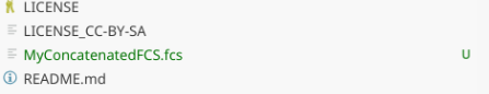
.
Which, as always, for sanity check when working with your own functions, its always best to double check everything stored correctly and opens as you will anticipate.
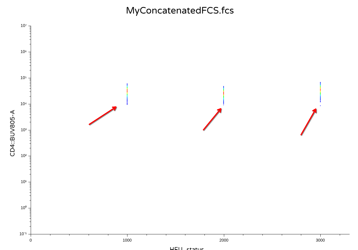
.
Likewise, similar to what we encountered with Downsampling, if we provide an improbably high-number for ‘DownsampleCount’, we just end up combining all our cells of interest for a given cell population, from each individual, together into a single file.
Concatenate(gs=SFC_GatingSet, subset="CD8+", addon="CD8", DownsampleCount=10000000,
  desiredCols=c("name", "condition", "infant_sex", "HEU_status"), returnType="flowframe")
flowFrame object 'MyConcatenatedFCS.fcs'
with 7159 cells and 47 observables:
name desc range minRange maxRange
$P1 Time NA 896744 0 896744
$P2 SSC-W NA 4194303 0 4194303
$P3 SSC-H NA 4194303 0 4194303
$P4 SSC-A NA 4194303 0 4194303
$P5 FSC-W NA 4194303 0 4194303
... ... ... ... ... ...
$P43 AF-A NA 4194275 -111 4194275
$P44 name NA 2001 1000 3000
$P45 condition NA 1 1000 1000
$P46 infant_sex NA 1001 1000 2000
$P47 HEU_status NA 2001 1000 3000
555 keywords are stored in the 'description' slotR
.
Over the course of today, we created two large functions, Downsampling() and Concatenate(), plus several helper functions. While currently active in our environment, what if we want to use them for a different project on another day? What would be the best way to make them available.
.
One approach to handling this issue I frequently encounter is placing your own functions within individual code blocks at the beginning of your .qmd file, so that they get activated in your local environment from the start of the process. However, if the functions are lengthy, this ends up occupying substantial portion of the document, which is less than ideal.
.
The approach we will be using for the next several weeks of the course is to place the completed functions in their own respective .R files files, all kept together in their own R folder within our working directory. For today’s functions, this would looks like this
.
Subsequently, when we need to load all these functions into our local environment, all we need to do is provide the file paths to walk alongside source() in order to activate all the .R files, making the functions they contain within available to us.
.
To load all these functions to our active environment, for the next several sessions, we would only need to use the source() function providing the path to the folder. This in turn will load in all the function .R files we have created, making their contents available to us in R for subsequent use. We will explore how this approach can be useful in context over the next several weeks.
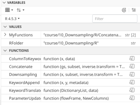
Discussion
.
In this session, we picked up where we left off on Week 09 and continued to gain additional experience with building useful functions, primarily in context of working through the assembly of our Downsampling() function, which we used successfully to both downsample and export particular cell types of interest out of our GatingSet objects. This in turn enabled the creation of a nested function Concatenate(), which provides us the ability to combine these outputs into a single .fcs, with the option of adding additional metadata columns.
.
Beyond the “building coding mindsets” and “function creation practice” aspects, these tools sets will prove quite useful when we start encountering more of the high-dimensional and unsupervised analysis content, both in terms of generating the right outputs needed to pass to these algorithms, but also that many of the steps we did today directly translate to the process of pipeline assembly. Which makes sense, as systematically working your way through a problem, converting outputs to inputs for the next function, is essentially what a pipeline does.
.
One thing to note for Concatenate, today, we only combined files together that were all acquired on the same day, and unmixed at the same time. Especially when it comes to Spectral Flow Cytometry experiments, things can vary a bit across experiment days, which when sufficiently different enough can result in batch effects for downstream unsupervised analytical algorithms. Consequently, when we get to the normalization week, we will need to modify our workflow to account for these adjustments before we concatenate everything together.
.
On the docket for next time, we will start to see where R gets its reputation as a statistical powerhouse, as we learn how to tidy our GatingSet gate counts appropiately so that they can be used for statistical significance testing. In the process, we learn how to pipe these outputs directly to ggplot plots for use in publication figures, as well as assemble pdfs and to allow for rapid screening. If all goes well, the days of copying and paste-ing columns from an excel file over to your subscription-based statistical analysis software may soon be a distant memory.

Additional Resources
Conditionals We used several additional conditionals today (if, ifelse, else), so would be helpful to explore some additional details on how these work.
De Novo Software - FCS Express: HD Data Analysis Part4 Downsampling Part of their High-dimensional analysis series, explores some additional ways to prioritize the downsampled cells depending on what your goal is (which are worth considering as we go along)
Advanced R: Dynamic Lookup One of the odd behaviors of functions that takes some getting used to, what does your function see or not see in terms of values? And what gets priority?
Take-home Problems
Problem 1
Load a dataset into R, gate it however you like, and then export out a population of interest as their own .fcs files. Open them in either Floreada.io or the commercial software of your choice, and take a screenshot of how they look by two markers of interest.
Problem 2
In the example for Downsampling() we only changed one keyword (GUID), after substituting in our desired addon right before the .fcs. Since keyword use might vary by manufacturer, create a couple additional arguments for Downsampling() that allow you to change out the values for some additional keywords.
Problem 3
Trickier - After concatenating out an .fcs file for a cell subset of your choice, reload it back into R, extract out both the exprs matrix, and the description list. Using the keywords that got added, figure out a way using dplyr to revert the numeric keys (denoted by “_key”) in the exprs matrix back to their original character values as recorded in the keywords.