Luciernaga Integration - Unstained
2026-08-30



For the YouTube recording, see here
For screen-shot slides, click here
Background
.
Due to the sheer number of plotly ggplotly() interactive plots that the website would need to load if we had visualized all the LuciernagaIntegration() plots for the 29-fluorophore panel (plus unstained controls) in one go, we have broken the exploration into smaller chapters. This walk-through if for the Unstained controls.
.
- To return to the main walk-through (including UV fluorophores), click here
- For the violet fluorophore walk-through, click here
- For the blue fluorophore walk-through, click here
- For the yellow-green fluorophore walk-through, click here
- For the red fluorophore walk-through, click here
- For the unstained samples walk-through, click here
Walk-through
Set Up
.
Attach your R packages to the local environment via the library() call.
.
Designate your file paths to the storage and output folder locations.
.
Bring in the pre-gated GatingSet object (which was carried out as part of the Set Up walkthrough).
.
We can then double check the existing gates.
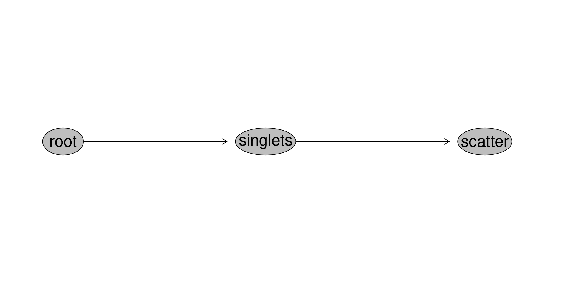
.
The last component we will need to run LuciernagaIntegration() wrapper function is the template data.frame. Since we are just looking at the unstained unmixing controls, this doesn’t need to be as highly detailed as the one we used for the single-color unmixing controls, so we can just generate out a generic one using mutate().
                                                 name  Type Fluorophore
1   DTR_2023_ILT_01-INF052-Ctrl_Unstained.1235650.fcs Cells     scatter
2 DTR_2023_ILT_01-ND006_v1-Ctrl_Unstained.1235671.fcs Cells     scatter
3  DTR_2023_ILT_01-ND006_v1-PMA_Unstained.1235672.fcs Cells     scatter
           Antigen Detector      Negative
1 Autofluorescence       V7 NoSubtraction
2 Autofluorescence       V7 NoSubtraction
3 Autofluorescence       V7 NoSubtraction
.
And with that, we are set!
Unstained Controls
.
For spectral flow cytometry, our cell unstained unmixing controls serve two main purposes. One is their use in subtracting out the background from the cell single-color unmixing controls, leaving in theory just the fluorophore signal for incorporation into the signature matrix. The second is that the unstained signature itself can also be provided to the unmixing matrix, allowing us to account for any autofluorescence signal that might be present, reducing the likelihood that the unaccounted for signal contribution ends up being misattributed to one of our fluorophores, which could result in an unmixing error.
.
Often in spectral flow cytometry, especially when working with peripheral blood mononuclear cells (PBMCs), we assume that only one unstained autofluorescence signature is present across our cell population of interest. Autofluorescence of individual cells is driven by the expression of a mix of biological molecules (ranging from amino acids like tryptophan, to intermediates like NADPH, cyclic molecules, and actin). A shared autofluorescence signature ultimately is the background signal of cells that share relative proportions of these intracellular autofluorescent molecules.
.
However, an increased expression of one autofluorescent molecule, or the production of a novel autofluorescent molecule with a different emission pattern has the potential to drive the appearance of additional discernable signature(s). Such a signature would be unaccounted for within the unmixing matrix if relying on just the “average signature”. The unmixing matrix would consequently be incomplete, with the additional signal being misattributed to other fluorophores, introducing unmixing errors (characteristically defined by distorted appearance and extreme negative values). Likewise, if an additional autofluorescent signature is included in a matrix when it is not present (or needed), it can hamper resolution for the other fluorophores with which it shares peaks (as we will cover in the Stain Reduction Index walkthrough in a couple weeks).
.
The Luciernaga package implements one approach at trying to systematically characterize the autofluorescences that are present across cells in our unstained samples. While not fully automating the decision making, it can allow us to more easily identify and isolate autofluorescent signature variants in our cell populations of interest that might be worth including as their own autofluorescent tags in scenarios where multiple-autofluorescences are present.
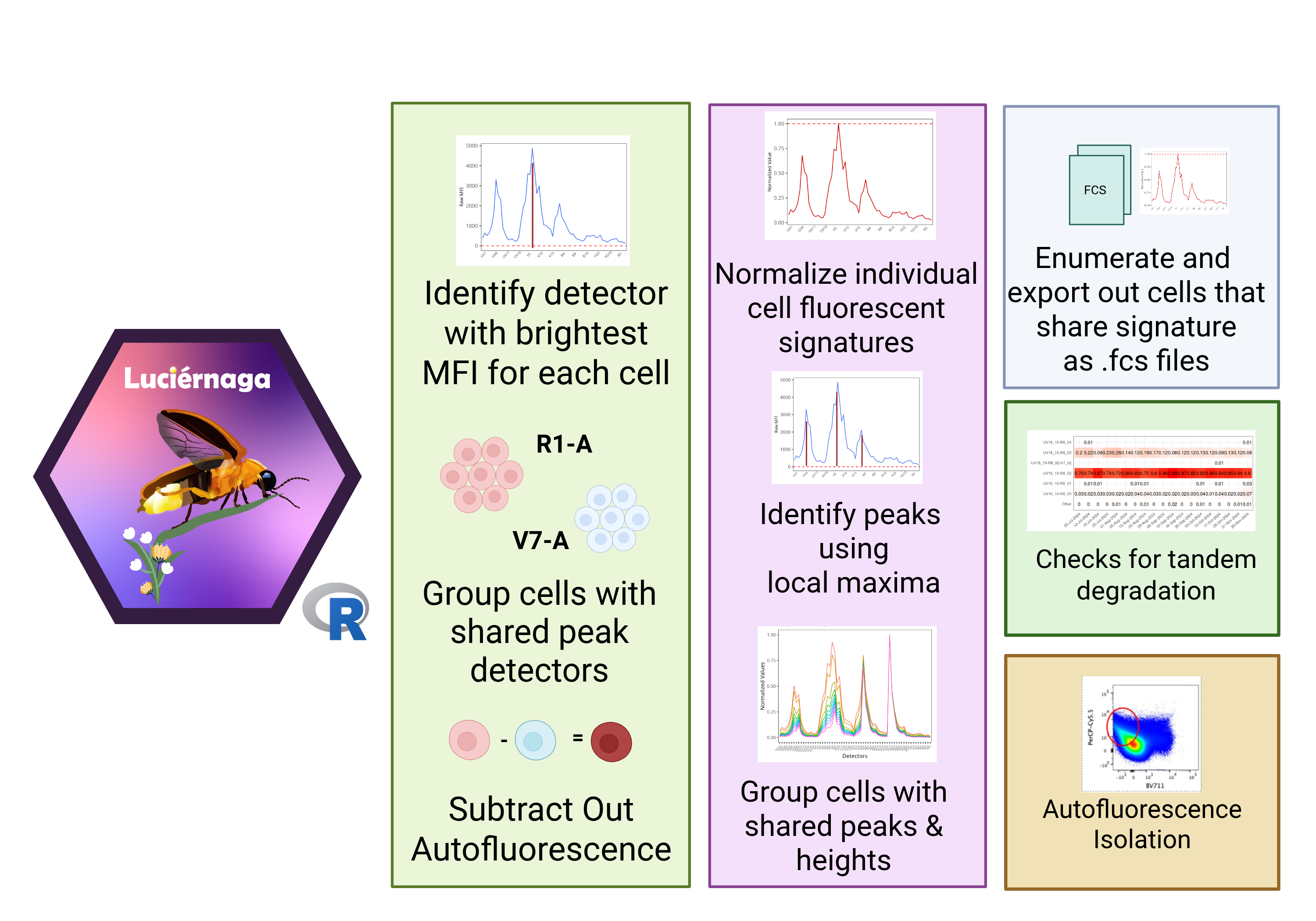
.
For this walk-through, we will examine both Cord and Peripheral blood mononuclear cells (CBMC, PBMC), at baseline and following PMA-ionomycin, to kick-start the process of how to use Luciernaga for troubleshooting for simpler cases (before encountering more complicated heterogeneous autofluorescence issues in later weeks).
CBMC
INF052 Ctrl
.
To run LuciernagaIntegration(), we need to provide our GatingSet object, and from the template the corresponding row for our specimen of interest. Checking the template, we can see that the CBMC specimen (INF052_Ctrl) is in the first row, so we can accesss it via adding [1,] after the template name to subset it. The main thing to remember, since this is an unstained unmixing control, we need to set “Unstained” argument equal to TRUE, otherwise the function will attempt to subtract background as it would for the single-color unmixing controls.
.
First off, we can check the “LinearSlices” output, to see if there would have been any differences in retrieved normalized signatures if we had split our gated cells into 10% bins of increasing MFI for the peak “V7-A” detector.
.
Overall, for our CBMC specimen, we see minor differences across the board, especially compared to what we have encountered previously for fluorophores. The dimmer 10% bins do have slightly more “B3-A” signal contribution compared to the “V7-A” detector than what we see for the brighter MFI bins. What about if we had used LuciernagaQC() and grouped normalized signatures of individual cells on the basis of shared peaks of similar heights?
.
At this point, we start encountering some of the autofluorescence variation on the per cell level, which can give everything a fuzzy caterpillar appearance. Beyond biological variability, some of the more erratic signals are partially due to instrumental noise introducing measurement error on individual detector, alongside low cell counts for that particular signature (which after the median results in the small spikes).
.
To see how this looks like overall, lets see where the median measurements end up based on our QC_Amalgamate() output.
.
Within our unstained cells in the “scatter” gate, we can see most are uniform for “V7-A” detector, but there is variable contribution to the signatures present for both “UV7-A” and “B3-A” (having values greater than 60% of the peak “V7-A” detector). Additionally, there is some smaller variation noticeable around both “V5-A” and “V10-A”. Lets focus on the UV7-A” and “B3-A” differences, and try to get an understanding of how abundant they might actually be across the signature variants.
.
We can start this process by first checking the “ProportionPlot” output.
.
Across the board, all signatures have “V7-A” as their peak detector. Looking at the populations with significant amounts of cells present (not 0%), most have their secondary peak on “B3-A”, with a dimmer third peak for “UV7-A” (except for 1% found in the V7_10-B3_04-UV8_05).
.
For this CBMC specimen, whatever autofluorescent molecule being made has a bit more of a “blue” contribution. If we look at unstained cells with “B3-A” contribution >60% of the “V7-A” peak detector height, it looks to be around 5% (main representative being “V7_10-B3_07-UV8_04”). For “UV7-A”, signatures with >50% of the “V7-A” peak detector are rather rare, with no individual signature crossing the 1% threshold.
.
Checking the cosine plot, we can see that overall, the various signatures are mostly similar to each other, with a few exceptions.
.
For now, lets grab a representative signature from a few of the main similar “blocks” that are visible, and compare how these signatures differ from the autofluorescent-similar fluorophores in our panel.
      Fluorophore ID_V7_10-B3_06-UV8_03 ID_V7_10-B3_03-UV8_03
1           BV510                  0.85                    NA
2  Spark Blue 550                  0.57                    NA
3          BUV496                  0.44                    NA
4           BV510                    NA                  0.90
5          BUV496                    NA                  0.45
6  Spark Blue 550                    NA                  0.43
7           BV510                    NA                    NA
8          BUV496                    NA                    NA
9  Spark Blue 550                    NA                    NA
10          BV510                    NA                    NA
11 Spark Blue 550                    NA                    NA
12         BUV496                    NA                    NA
   ID_V7_10-B3_04-UV8_05 ID_Average
1                     NA         NA
2                     NA         NA
3                     NA         NA
4                     NA         NA
5                     NA         NA
6                     NA         NA
7                   0.88         NA
8                   0.50         NA
9                   0.49         NA
10                    NA       0.87
11                    NA       0.53
12                    NA       0.46
.
We will explore how these differences impact the unmixing of autofluorescence-similar fluorophores when we use these different unstained signatures for unmixing during Week 15.
Pass
Overall, most of the signatures appear to be normal/typical for fixed cells, with all the variants sharing primary peak detector (“V7-A”), but differing in height of their secondary (“B3-A”) and third peaks (“UV7-A”). Variant signatures that differed substantially in their heights for these secondary and tertiary peaks were relatively rare overall. So first impression, this would likely unmix normally using a single-unstained signature.
PBMC
ND006 Control
.
Next up, we switch from neonate CBMC to adult PBMC. Obviously, different donor and processing time, but we might also expect to see some differences that might arise from different metabolism, so its worth keeping an eye on how the secondary and tertiary peak heights compare with the previous example.
.
We can start off by first running LuciernagaIntegration() using the GatingSet object, and the corresponding row for the specimen of interest in the template. The main thing to remember, since this is an unstained unmixing control, we need to set “Unstained” argument equal to TRUE.
.
First off, we can check the “LinearSlices” output, to see if there would have been any differences in retrieved normalized signatures if we had split our gated cells into 10% bins of increasing MFI for the peak “V7-A” detector.
.
Rather minor differences across the board, especially compared to what we have encountered previously for fluorophores. Once again, cells with dimmer MFI appear to have slightly more of a “B3-A” contribution. What about if we had used LuciernagaQC() and grouped normalized signatures of individual cells on the basis of shared peaks of similar heights?
.
We continue to get back fuzzy caterpillars (as we are starting to get used to seeing for our unstained cells). However, contrasting to the CBMC specimen above, there appears to be substantially more “UV7-A” signal than “B3-A”, with the “UV7-A” peak variation appearing to nearly match the height of the primary “V7-A” detector in some cases.
.
Lets see where the median measurements end up based on our QC_Amalgamate() output.
.
Within our unstained cells in the “scatter” gate, we can see most are uniform for “V7-A” detector, but there is quite a bit of variation present in the “UV7-A” detector. Contrasting to CBMC, the “UV7-A” is the secondary peak for most cells, with the “B3-A” being dimmer overall. Lets try to get an understanding of how abundant these variant signatures are across the cells in our gate, by checking the “ProportionPlot” output.
.
The majority of cells appear to be “V7-A” as their peak detector, with the respective heights of the secondary “UV7-A” and tertiary “B3-A” peak ranging from 0.4 to 0.5 (64% of all cells).
.
So for unstained cells featuring a “UV7-A” contribution >60% of the “V7-A” peak detector height, it looks to be around 4% (main representative being “V7_10-UV8_07-B3_05”). For “B3-A”, signatures with >60% of the “V7-A” peak detector are extremely rare, with no individual signature crossing the 1% threshold.
.
If we check the Cosine plot, we can see these examples in action.
.
We might also be interested in seeing how similar it might be to our autofluoresce-like fluorophores.
Pass
Overall, the majority of the cells (65%) share similar autofluorescence, with a primary peak of “V7”, with secondary peaks of “UV7” and “B3” around 50% of the primary peak.
Overall, compared to the previous CBMC specimen, the secondary peak is shifted toward “UV7” instead of “B3”, which might impact interchangeability if we tried using it to subtract background.
We however noted quite a bit of variability for the “UV7” peak height, in some cases the peak matched or surpassed the “V7” peak. This might make this specimen useful for delineating when an autofluorescence becomes sufficiently different that it merits addition as its own autofluorescence tag.
ND006 PMA
.
And last in today’s examples, we have the ND006 PBMC donors unstained cells that were activated with PMA-ionomycin for 6 hours. We will see if this strong activation has caused any metabolic shifts that might be noticeable at the autofluorescence signature level.
.
We can start off by first running LuciernagaIntegration() using the GatingSet object, and the corresponding row for the specimen of interest in the template. The main thing to remember, since this is an unstained unmixing control, we need to set “Unstained” argument equal to TRUE.
.
First off, we can check the “LinearSlices” output, to see if there would have been any differences in retrieved normalized signatures if we had split our gated cells into 10% bins of increasing MFI for the peak “V7-A” detector.
.
Rather minor differences across the board, especially compared to what we have encountered previously for fluorophores. Still noting minor shifts in the “B3-A” height for the lower 10% bins. What about if we had used LuciernagaQC() and grouped normalized signatures of individual cells on the basis of shared peaks of similar heights?
.
Still getting fuzzy caterpillars (as we would anticipate for unstained controls). In this case, looks very similar to what we saw for the control ND006, with a primary peak on “V7-A”, secondary peak (with a lot of variation) on “UV7-A”, smaller tertiary peak for “B3-A”. Lets see where the median measurements end up based on our QC_Amalgamate() output.
.
The majority of cells appear to be “V7-A” as their peak detector, with the respective heights of the secondary “UV7-A” and tertiary “B3-A” peak.. This appears to be pretty similar to what we saw for the control specimen of the donor as well, but shifted from the CBMC’s secondary peak at “B3-A”. Overall, still substantial variation for this donor in terms of the signatures contribution present on “UV7-A”
.
Lets check the “ProportionPlot” to see how these are distributed.
.
The majority of the unstained cells continued to have a primary peak of “V7”, with secondary and tertiary peaks on “UV7” and “B3” between 0.4 and 0.6 of the primary peak height (63%).
.
So for unstained cells with “UV7-A” contribution >60% of the “V7-A” peak detector height, it looks to be around 3% (main representative being “V7_10-UV8_07-B3_05”). For “B3-A”, signatures with >60% of the “V7-A” peak detector are extremely rare, with no individual signature crossing the 1% threshold.
.
If we check the Cosine plot, we can see that overall, the various signatures are mostly similar to each other, with a few exceptions.
.
Once again, we can see some of the rarer “UV7” peak cells that don’t make up 1% of the population, but contribute to the appearance of Blue in the plot. Lets grab a few of the representative fluorophores and compare how they are similar to our autofluoresce-like fluorophores.
      Fluorophore ID_V7_10-UV8_04-B3_04 ID_V7_10-UV8_08-B3_04
1           BV510                  0.90                    NA
2          BUV496                  0.50                    NA
3  Spark Blue 550                  0.48                    NA
4           BV510                    NA                  0.88
5          BUV496                    NA                  0.64
6  Spark Blue 550                    NA                  0.44
7           BV510                    NA                    NA
8          BUV496                    NA                    NA
9  Spark Blue 550                    NA                    NA
10          BV510                    NA                    NA
11         BUV496                    NA                    NA
12 Spark Blue 550                    NA                    NA
   ID_UV7_10-UV8_09-V7_07 ID_Average
1                      NA         NA
2                      NA         NA
3                      NA         NA
4                      NA         NA
5                      NA         NA
6                      NA         NA
7                    0.79         NA
8                    0.75         NA
9                    0.41         NA
10                     NA       0.89
11                     NA       0.51
12                     NA       0.51
Pass
Overall, similar autofluorescence profile for this PBMC donor in its activation condition compared to the control, with both being shifted toward the UV compared to the CBMC. While no immediately obvious shift is seen resulting for the PMA-ionomycin stimulation, it does look like the “UV7” variants with equal or greater height to the “V7” peak while rare are more widespread than for the previous control condition, and might be worth evaluating for their effect on the unmixing.
Redirects
.
Due to the sheer number of plotly ggplotly() interactive plots that the website would need to load if we had visualized all the LuciernagaIntegration() plots for the 29-fluorophore panel (plus unstained controls) in one go, we have broken the exploration into smaller chapters. This walk-through if for the Unstained controls.
.
- To return to the main walk-through (including UV fluorophores), click here
- For the violet fluorophore walk-through, click here
- For the blue fluorophore walk-through, click here
- For the yellow-green fluorophore walk-through, click here
- For the red fluorophore walk-through, click here
- For the unstained samples walk-through, click here
Additional Resources
Luciernaga Vignette - Reference Library
Luciernaga Vignette - Fluorescent Signatures