Luciernaga Integration
David Rach
2026-08-30



For the YouTube recording, see here
For screen-shot slides, click here
Background
.
In the previous bonus walk-through, we generated signature matrices for both our bead and cell single-color unmixing controls using the flowGate and Luciernaga R packages. The normalized fluorescent signatures were generated by extracting cells (or beads) that fell within our peak detector gates, taking the median measurement across each detector, subtracting out the equivalent background autofluorescence, and then normalizing (scaling) the values to range from 0 to 1. The normalized fluorescent signatures from all the fluorophores were then assembled together into a signature matrix.
.
Overall, this workflow is representative of the approach taken within most commercial softwares in the steps leading up to unmixing. Unfortunately, relying on a summary measurement (“median” in this case) often limits what we are able to perceive, and when it comes to the unmixing controls,there remains plenty of additional information that can be gleaned from the individual cells that are present.
.
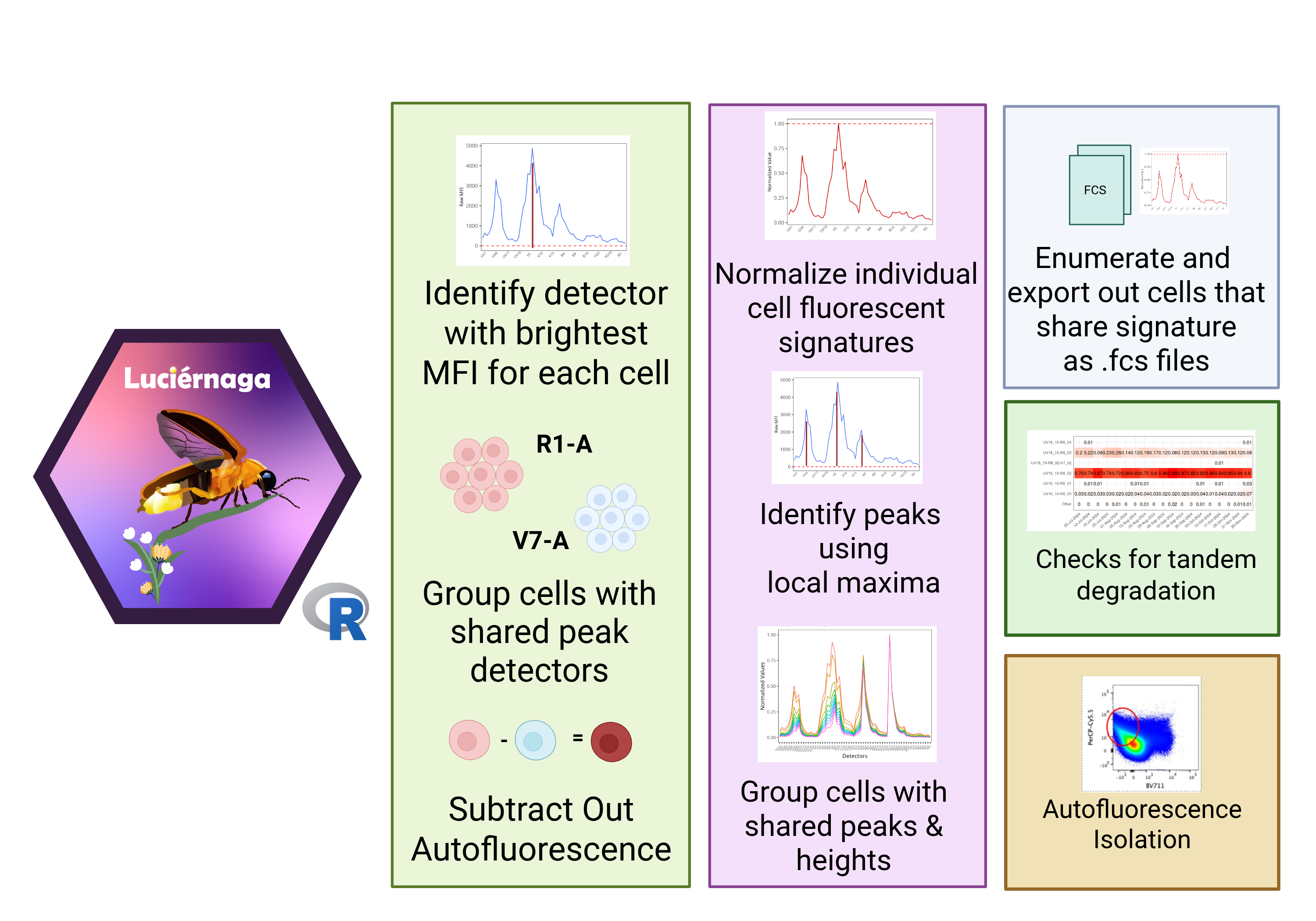
During Week 12, we showcased the use of the Luciernaga packages LuciernagaIntegration() wrapper function, which permitted grouping cells based on their individual normalized cell signatures based on shared peaks, of relatively same heights.
.
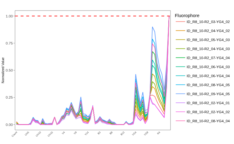
This approach proved useful, as it allowed us to identify the tandem degradation from APC-Fire 810 to APC that was occuring in the cell single-color controls (but strangely not the bead single-color control prepared from the same antibody vial).
.
In this walk-through, we will take a look at the other 28-fluorophores in the panel, and identify any other frequently encountered patterns that can be found when we look at our unmixing controls with such a granular view. We will also explore how to leverage this information to better inform which signatures we incorporate into the final fluorophore signature matrix for use in unmixing the full-stained samples.
Walk Through
Set Up
Retrieving GatingSet
.
Next up, specify the storage (currently containing our .fcs files) and output (currently containing our intermediate .gs folder) locations. If you are following the courses organization scheme, these would be in the “data” and “outputs” folders respectively.
.
With these file paths set up, lets proceed to load our CellSC_GatingSet back into the local environment from its .gs folder. This would be the “Amplified” version, where the peak detector gates had been created, checked and corrected.
.
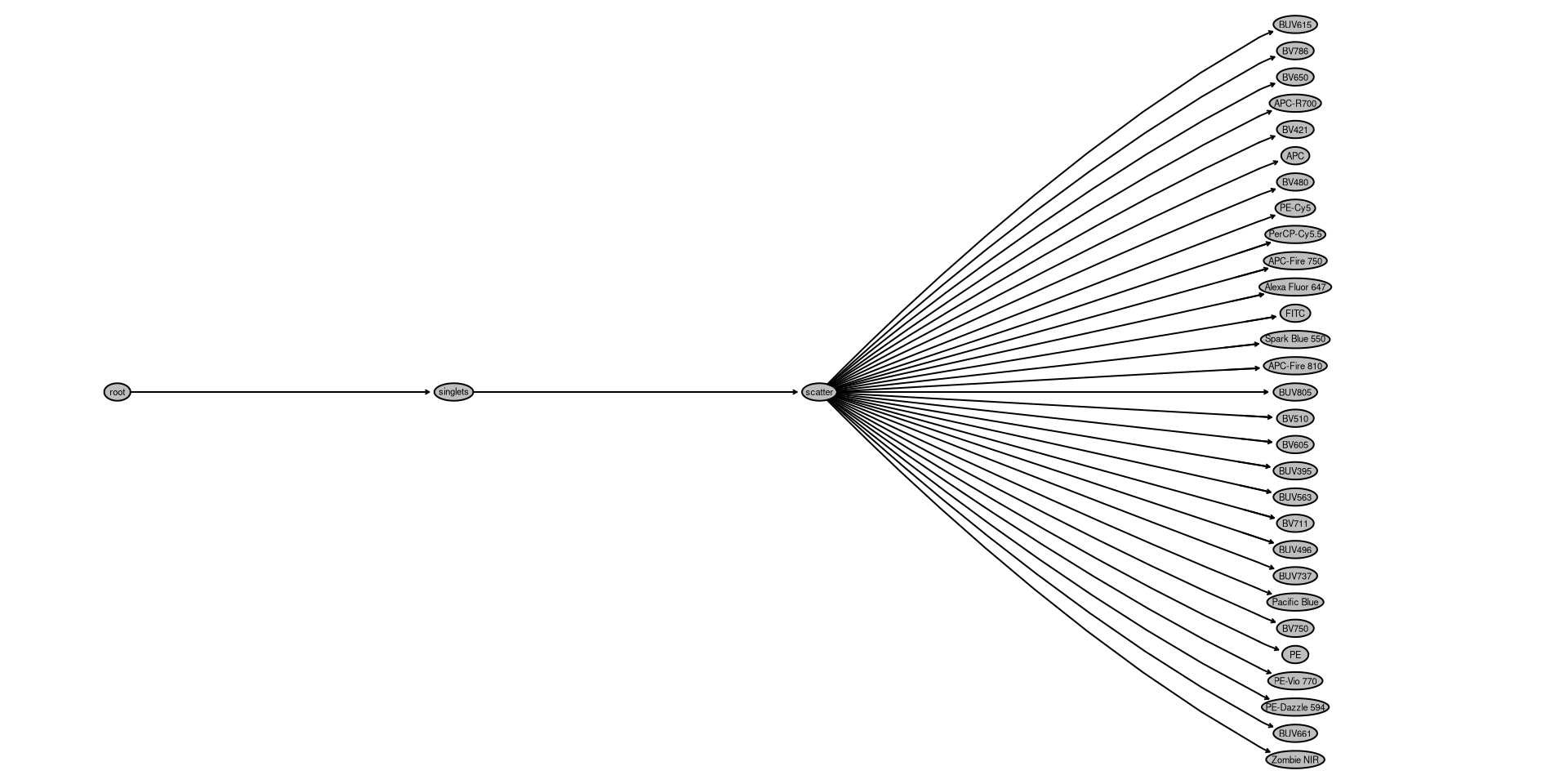
And lets go ahead and plot the gates, just to make sure everything remains as it should be.
Assembling Template
.
Since LuciernagaIntegration() wrapper function relies on the use of a template for matching the individual single-color control specimen with the corresponding peak detector gate, we can reasseble the template by retrieving the updated metadata using pData(). When re-retrieving metadata from a GatingSet, the metadata columns order may end up rearranged, so lets also reorganize the columns based on the expected order we previously had them in.
                                                                name
1 DTR_2023_ILT_01-Reference Group-DR_CCR4 BUV615 (Cells).1235678.fcs
2  DTR_2023_ILT_01-Reference Group-DR_CCR6 BV786 (Cells).1235679.fcs
3  DTR_2023_ILT_01-Reference Group-DR_CCR7 BV650 (Cells).1235680.fcs
  Fluorophore Antigen  Type Detector       Negative
1      BUV615    CCR4 Cells     UV10 PBMC_Unstained
2       BV786    CCR6 Cells      V15 PBMC_Unstained
3       BV650    CCR7 Cells      V11 PBMC_Unstained
.
We can also optionally remove the 3 samples that we previously choose not to investigate using the dplyr packages filter() function on the data.frame object. We can save this subsetted output as a new object/variable, “KeptCells”.
KeptCells <- Template |>
     filter(!name %in% "DTR_2023_ILT_01-Reference Group-DR_Dump_CD19 Pacific Blue (Cells).1235702.fcs") |>
     filter(!name %in% "DTR_2023_ILT_01-Reference Group-DR_Viability_PMA Zombie NIR (Cells).1235709.fcs") |>
filter(!name %in% "DTR_2023_ILT_01-Reference Group-DR_CD3 Alexa Fluor 488 (Cells).1235688.fcs") name
1 DTR_2023_ILT_01-Reference Group-DR_CCR4 BUV615 (Cells).1235678.fcs
2 DTR_2023_ILT_01-Reference Group-DR_CCR6 BV786 (Cells).1235679.fcs
3 DTR_2023_ILT_01-Reference Group-DR_CCR7 BV650 (Cells).1235680.fcs
4 DTR_2023_ILT_01-Reference Group-DR_CD107a APC-R700 (Cells).1235681.fcs
5 DTR_2023_ILT_01-Reference Group-DR_CD127 BV421 (Cells).1235682.fcs
6 DTR_2023_ILT_01-Reference Group-DR_CD16 APC (Cells).1235683.fcs
7 DTR_2023_ILT_01-Reference Group-DR_CD161 BV480 (Cells).1235684.fcs
8 DTR_2023_ILT_01-Reference Group-DR_CD25 PE-Cy5 (Cells).1235685.fcs
9 DTR_2023_ILT_01-Reference Group-DR_CD26 PerCP-Cy5.5 (Cells).1235686.fcs
10 DTR_2023_ILT_01-Reference Group-DR_CD27 APC-Fire 750 (Cells).1235687.fcs
11 DTR_2023_ILT_01-Reference Group-DR_CD3 Alexa Fluor 647 (Cells).1235689.fcs
12 DTR_2023_ILT_01-Reference Group-DR_CD3 FITC (Cells).1235690.fcs
13 DTR_2023_ILT_01-Reference Group-DR_CD3 Spark Blue 550 (Cells).1235691.fcs
14 DTR_2023_ILT_01-Reference Group-DR_CD38 APC-Fire 810 (Cells).1235692.fcs
15 DTR_2023_ILT_01-Reference Group-DR_CD4 BUV805 (Cells).1235693.fcs
16 DTR_2023_ILT_01-Reference Group-DR_CD45RA BV510 (Cells).1235694.fcs
17 DTR_2023_ILT_01-Reference Group-DR_CD56 BV605 (Cells).1235695.fcs
18 DTR_2023_ILT_01-Reference Group-DR_CD62L BUV395 (Cells).1235696.fcs
19 DTR_2023_ILT_01-Reference Group-DR_CD69 BUV563 (Cells).1235697.fcs
20 DTR_2023_ILT_01-Reference Group-DR_CD7 BV711 (Cells).1235698.fcs
21 DTR_2023_ILT_01-Reference Group-DR_CD8 BUV496 (Cells).1235699.fcs
22 DTR_2023_ILT_01-Reference Group-DR_CXCR3 BUV737 (Cells).1235700.fcs
23 DTR_2023_ILT_01-Reference Group-DR_Dump_CD14 Pacific Blue (Cells).1235701.fcs
24 DTR_2023_ILT_01-Reference Group-DR_IFNg BV750 (Cells).1235703.fcs
25 DTR_2023_ILT_01-Reference Group-DR_NKG2D PE (Cells).1235704.fcs
26 DTR_2023_ILT_01-Reference Group-DR_PD1 PE-Vio770 (Cells).1235705.fcs
27 DTR_2023_ILT_01-Reference Group-DR_TNFa PE-Dazzle594 (Cells).1235706.fcs
28 DTR_2023_ILT_01-Reference Group-DR_VD2 BUV661 (Cells).1235707.fcs
29 DTR_2023_ILT_01-Reference Group-DR_Viability Zombie NIR (Cells).1235708.fcs
Fluorophore Antigen Type Detector Negative
1 BUV615 CCR4 Cells UV10 PBMC_Unstained
2 BV786 CCR6 Cells V15 PBMC_Unstained
3 BV650 CCR7 Cells V11 PBMC_Unstained
4 APC-R700 CD107a Cells R4 PBMC_Activated_Unstained
5 BV421 CD127 Cells V1 PBMC_Unstained
6 APC CD16 Cells R1 CBMC_Unstained
7 BV480 CD161 Cells V5 PBMC_Unstained
8 PE-Cy5 CD25 Cells YG5 PBMC_Activated_Unstained
9 PerCP-Cy5.5 CD26 Cells B9 PBMC_Unstained
10 APC-Fire 750 CD27 Cells R7 PBMC_Unstained
11 Alexa Fluor 647 CD3 Cells R2 PBMC_Unstained
12 FITC CD3 Cells B2 PBMC_Unstained
13 Spark Blue 550 CD3 Cells B3 PBMC_Unstained
14 APC-Fire 810 CD38 Cells R8 CBMC_Unstained
15 BUV805 CD4 Cells UV16 PBMC_Unstained
16 BV510 CD45RA Cells V7 CBMC_Unstained
17 BV605 CD56 Cells V10 CBMC_Unstained
18 BUV395 CD62L Cells UV2 PBMC_Unstained
19 BUV563 CD69 Cells UV9 PBMC_Activated_Unstained
20 BV711 CD7 Cells V13 PBMC_Unstained
21 BUV496 CD8 Cells UV7 CBMC_Unstained
22 BUV737 CXCR3 Cells UV14 PBMC_Unstained
23 Pacific Blue Dump_CD14 Cells V3 PBMC_Monocyte_Unstained
24 BV750 IFNg Cells V14 PBMC_Activated_Unstained
25 PE NKG2D Cells YG1 PBMC_Unstained
26 PE-Vio 770 PD1 Cells YG9 CBMC_Unstained
27 PE-Dazzle 594 TNFa Cells YG3 PBMC_Activated_Unstained
28 BUV661 VD2 Cells UV11 PBMC_Unstained
29 Zombie NIR Viability Cells R6 CBMC_Dead_UnstainedRearranging by Detector
.
Before diving too far in, you may notice the rows in our current template are not exactly ordered in terms of the laser and emission wavelength of the respective fluorophores. We can fix this setting factor() on the detector column (providing the correct detector order via the levels argument). At that point, we can use the dplyr packages arrange() function to re-shuffle the rows to match the designated factor ordering.
DetectorOrder <- c("UV1", "UV2", "UV3", "UV4", "UV5", "UV6", "UV7", "UV8",
               "UV9", "UV10", "UV11", "UV12", "UV13", "UV14", "UV15", "UV16",
               "V1", "V2", "V3", "V4", "V5", "V6", "V7", "V8",
               "V9", "V10", "V11","V12", "V13", "V14", "V15", "V16",
               "B1", "B2", "B3", "B4", "B5", "B6", "B7", "B8",
               "B9", "B10", "B11", "B12", "B13", "B14",
               "YG1", "YG2", "YG3", "YG4", "YG5", "YG6", "YG7", "YG8", "YG9", "YG10",
               "R1", "R2", "R3", "R4", "R5", "R6", "R7", "R8")

KeptCells$Detector <- factor(KeptCells$Detector, levels=DetectorOrder)

KeptCells <- KeptCells |> arrange(Detector) name
1 DTR_2023_ILT_01-Reference Group-DR_CD62L BUV395 (Cells).1235696.fcs
2 DTR_2023_ILT_01-Reference Group-DR_CD8 BUV496 (Cells).1235699.fcs
3 DTR_2023_ILT_01-Reference Group-DR_CD69 BUV563 (Cells).1235697.fcs
4 DTR_2023_ILT_01-Reference Group-DR_CCR4 BUV615 (Cells).1235678.fcs
5 DTR_2023_ILT_01-Reference Group-DR_VD2 BUV661 (Cells).1235707.fcs
6 DTR_2023_ILT_01-Reference Group-DR_CXCR3 BUV737 (Cells).1235700.fcs
7 DTR_2023_ILT_01-Reference Group-DR_CD4 BUV805 (Cells).1235693.fcs
8 DTR_2023_ILT_01-Reference Group-DR_CD127 BV421 (Cells).1235682.fcs
9 DTR_2023_ILT_01-Reference Group-DR_Dump_CD14 Pacific Blue (Cells).1235701.fcs
10 DTR_2023_ILT_01-Reference Group-DR_CD161 BV480 (Cells).1235684.fcs
11 DTR_2023_ILT_01-Reference Group-DR_CD45RA BV510 (Cells).1235694.fcs
12 DTR_2023_ILT_01-Reference Group-DR_CD56 BV605 (Cells).1235695.fcs
13 DTR_2023_ILT_01-Reference Group-DR_CCR7 BV650 (Cells).1235680.fcs
14 DTR_2023_ILT_01-Reference Group-DR_CD7 BV711 (Cells).1235698.fcs
15 DTR_2023_ILT_01-Reference Group-DR_IFNg BV750 (Cells).1235703.fcs
16 DTR_2023_ILT_01-Reference Group-DR_CCR6 BV786 (Cells).1235679.fcs
17 DTR_2023_ILT_01-Reference Group-DR_CD3 FITC (Cells).1235690.fcs
18 DTR_2023_ILT_01-Reference Group-DR_CD3 Spark Blue 550 (Cells).1235691.fcs
19 DTR_2023_ILT_01-Reference Group-DR_CD26 PerCP-Cy5.5 (Cells).1235686.fcs
20 DTR_2023_ILT_01-Reference Group-DR_NKG2D PE (Cells).1235704.fcs
21 DTR_2023_ILT_01-Reference Group-DR_TNFa PE-Dazzle594 (Cells).1235706.fcs
22 DTR_2023_ILT_01-Reference Group-DR_CD25 PE-Cy5 (Cells).1235685.fcs
23 DTR_2023_ILT_01-Reference Group-DR_PD1 PE-Vio770 (Cells).1235705.fcs
24 DTR_2023_ILT_01-Reference Group-DR_CD16 APC (Cells).1235683.fcs
25 DTR_2023_ILT_01-Reference Group-DR_CD3 Alexa Fluor 647 (Cells).1235689.fcs
26 DTR_2023_ILT_01-Reference Group-DR_CD107a APC-R700 (Cells).1235681.fcs
27 DTR_2023_ILT_01-Reference Group-DR_Viability Zombie NIR (Cells).1235708.fcs
28 DTR_2023_ILT_01-Reference Group-DR_CD27 APC-Fire 750 (Cells).1235687.fcs
29 DTR_2023_ILT_01-Reference Group-DR_CD38 APC-Fire 810 (Cells).1235692.fcs
Fluorophore Antigen Type Detector Negative
1 BUV395 CD62L Cells UV2 PBMC_Unstained
2 BUV496 CD8 Cells UV7 CBMC_Unstained
3 BUV563 CD69 Cells UV9 PBMC_Activated_Unstained
4 BUV615 CCR4 Cells UV10 PBMC_Unstained
5 BUV661 VD2 Cells UV11 PBMC_Unstained
6 BUV737 CXCR3 Cells UV14 PBMC_Unstained
7 BUV805 CD4 Cells UV16 PBMC_Unstained
8 BV421 CD127 Cells V1 PBMC_Unstained
9 Pacific Blue Dump_CD14 Cells V3 PBMC_Monocyte_Unstained
10 BV480 CD161 Cells V5 PBMC_Unstained
11 BV510 CD45RA Cells V7 CBMC_Unstained
12 BV605 CD56 Cells V10 CBMC_Unstained
13 BV650 CCR7 Cells V11 PBMC_Unstained
14 BV711 CD7 Cells V13 PBMC_Unstained
15 BV750 IFNg Cells V14 PBMC_Activated_Unstained
16 BV786 CCR6 Cells V15 PBMC_Unstained
17 FITC CD3 Cells B2 PBMC_Unstained
18 Spark Blue 550 CD3 Cells B3 PBMC_Unstained
19 PerCP-Cy5.5 CD26 Cells B9 PBMC_Unstained
20 PE NKG2D Cells YG1 PBMC_Unstained
21 PE-Dazzle 594 TNFa Cells YG3 PBMC_Activated_Unstained
22 PE-Cy5 CD25 Cells YG5 PBMC_Activated_Unstained
23 PE-Vio 770 PD1 Cells YG9 CBMC_Unstained
24 APC CD16 Cells R1 CBMC_Unstained
25 Alexa Fluor 647 CD3 Cells R2 PBMC_Unstained
26 APC-R700 CD107a Cells R4 PBMC_Activated_Unstained
27 Zombie NIR Viability Cells R6 CBMC_Dead_Unstained
28 APC-Fire 750 CD27 Cells R7 PBMC_Unstained
29 APC-Fire 810 CD38 Cells R8 CBMC_Unstained.
An added benefit of this means we can now use R notation for rows ([1,], [2,], etc.) to sequentially isolate out from the panel GatingSet just the individual fluorophores we want to work with by providing smaller versions of the actual template.
Cell Single-Color Controls
.
Before getting started, lets quickly recall which fluorophores that are present in this 29-fluorophore panel
| D | WV | Fluorophore | Antigen | D | Fluorophore | Antigen | D | Fluorophore | Antigen | D | Fluorophore | Antigen | D | Fluorophore | Antigen |
|---|---|---|---|---|---|---|---|---|---|---|---|---|---|---|---|
| UV1 | 373 | ||||||||||||||
| UV2 | 388 | BUV395 | CD62L | ||||||||||||
| UV3 | 428 | V1 | BV421 | CD127 | |||||||||||
| UV4 | 443 | V2 | |||||||||||||
| UV5 | 458 | V3 | Pacific Blue | Dump_CD14 | |||||||||||
| UV6 | 473 | V4 | |||||||||||||
| 508 | V5 | BV480 | CD161 | B1 | |||||||||||
| UV7 | 514 | BUV496 | CD8 | ||||||||||||
| 525 | V6 | B2 | FITC | CD3 | |||||||||||
| UV8 | 542 | V7 | BV510 | CD45RA | B3 | Spark Blue 550 | CD3 | ||||||||
| 577 | YG1 | PE | NKG2D | ||||||||||||
| 581 | V8 | B4 | |||||||||||||
| UV9 | 582 | BUV563 | CD69 | ||||||||||||
| 598 | V9 | B5 | YG2 | ||||||||||||
| UV10 | 613 | BUV615 | CCR4 | ||||||||||||
| 615 | V10 | BV605 | CD56 | B6 | YG3 | PE-Dazzle 594 | TNFa | ||||||||
| UV11 | 662 | BUV661 | VD2 | V11 | BV650 | CCR7 | B7 | YG4 | R1 | APC | CD16 | ||||
| 679 | B8 | YG5 | PE-Cy5 | CD25 | R2 | Alexa Fluor 647 | CD3 | ||||||||
| UV12 | 695 | V12 | B9 | PerCP-Cy5.5 | CD26 | YG6 | R3 | ||||||||
| UV13 | 718 | V13 | BV711 | CD7 | B10 | YG7 | R4 | APC-R700 | CD107a | ||||||
| 738 | B11 | R5 | |||||||||||||
| UV14 | 750 | BUV737 | CXCR3 | V14 | BV750 | IFNg | YG8 | ||||||||
| 760 | B12 | R6 | Zombie NIR | Viability | |||||||||||
| UV15 | 781 | V15 | BV786 | CCR6 | B13 | YG9 | PE-Vio 770 | PD1 | R7 | APC-Fire 750 | CD27 | ||||
| UV16 | 812 | BUV805 | CD4 | V16 | B14 | YG10 | R8 | APC-Fire 810 | CD38 |
.
As we start to evaluate fluorophore signatures, an important thing to remember is that what we (and our cytometers) perceive as brightness is a combination of
.
- The antigen density on the cell surface that our antibody-conjugated fluorophores will bind to.
.
- The individual fluorophores capacity to emit photons back when the respective laser excites it (as well as our instruments ability to capture this emmitted signal)
.
- Some variable amount of background autofluorescence (from either our cell or bead)
.
- Some additional amount of uncertainty or noise for good measure from various sources.
.
As we consider signature variants while profiling the normalized fluorescent signatures of individual cells, its often useful to try to mentually contextualize what we are seeing in light of these factors listed above. We will revisit these points in finer detail as we navigate through this walk-through. But for now, lets get started!
Ultra Violet
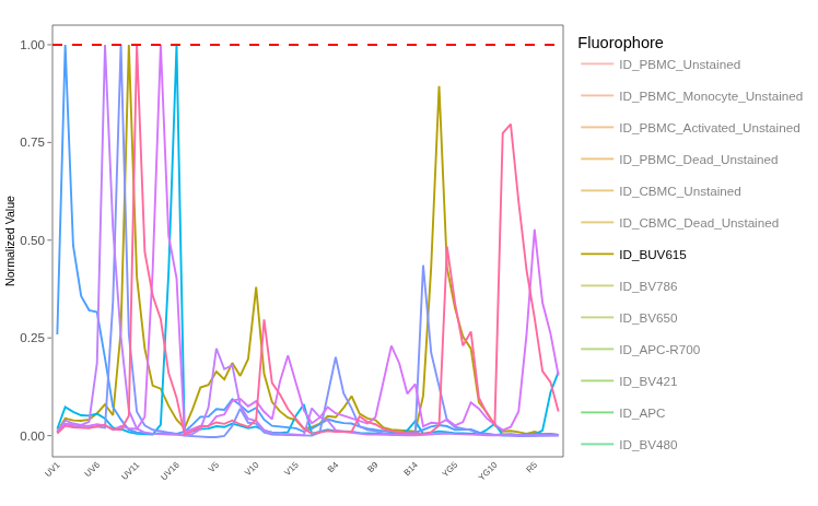
BUV395
.
Since it is located in the first row of our “data.frame”, we can subset it out from the broader “KeptCells” template using “[1,]”. We can pass this subsetted template alongside our GatingSet object to the LuciernagaIntegration() wrapper function for processing.
.
The LuciernagaIntegration() function in turn returns to us a list object.
.
If we run names(), we can see the actual contents appear to be a mix of both “data.frames” and “ggplot plots”, corresponding to the various Luciernaga functions that were run by the wrapper.
.
This allows us to quickly visualize via the different options, while retaining the ability to subsequently retrieve the underlying data for subsequent downstream analysis steps.
.
We can start by retrieving the output of Luciernaga_LinearSlices(), which is stored under the “LinearSlices_Plot” entry. This function splits the gated region into 10% bins across, and returns the averaged normalized signature for the cells that are present within each of the bins. This plot in turn can be passed to plotly’s ggplotly() function to render it interactive.
.
Across the board, it doesn’t appear that the normalized signature has changed substantially, as looking across the various bins the signatures appear mostly consistent.
.
Having noted this, we can next check the stored plot present under “LuciernagaQC_Signatures”, which is the wrapped return from the LuciernagaQC() function that orchestrates the grouping of cells based on their individual normalized signatures based on peak detector location and relative height.
.
Using this approach, we find the same signature that was seen by the prior approach (“UV2_10”, consisting of a single emission peak located at the “UV2” detector, i.e. normalized height of 1.00). However, we also retrieved a couple additional signature variants, with the presence of secondary peaks at the “V7” detector, that are of different heights relative to the peak “UV2” detector (“V7_02” ~ 20% height of UV2, “V7_03” ~ 30% height of UV2).
.
Given the location (“V7-A”), it is likely that this new peak in these two variant signatures is residual autofluorescence that wasn’t fully subtracted out for their individual cells.
.
While we can see there are variant signatures with residual autofluorescence present, this doesn’t tell us much information about how prevalent they might be. Within our returned list, we also have a “ProportionPlot” that tells us how the cells within our gated region where distributed between the signature variants.
.
In this case, around 80% of the cells had the standard signature, while 20% of the cells were better represented by the other two variant signatures. Within our LuciernagaIntegration() output list we also get back the QC_Amalgamate() functions output under the “LuciernagaQC_AmalgamatedPlot” entry. This will visualize all the signature variants, while also showing where the overall median signature would end up.
.
As we can see, in this case the “Average” and “UV2_10” signatures are practically indistinguishable, with the contribution of the variant signatures not affecting the overall shape of the signature.
.
Going back to the list, lets retrieve the underlying data for our plot (“AveragedSignature_Data”)
       Cluster     UV1-A UV2-A     UV3-A     UV4-A     UV5-A     UV6-A
1       UV2_10 0.2513256     1 0.4821444 0.3425974 0.3085460 0.2839456
2 UV2_10-V7_02 0.2548048     1 0.5012830 0.3707769 0.3268080 0.3237033
3 UV2_10-V7_03 0.2885756     1 0.4999609 0.3825903 0.3427424 0.3435264
4      Average 0.2513256     1 0.4821444 0.3425974 0.3085460 0.2839456
      UV7-A      UV8-A      UV9-A     UV10-A     UV11-A      UV12-A      UV13-A
1 0.1504531 0.04285274 0.01264474 0.00106715 0.00000000 0.000000000 0.000000000
2 0.2223727 0.09474590 0.06470829 0.02349097 0.01225132 0.009411968 0.004118347
3 0.2744997 0.14037336 0.09838418 0.03500394 0.02968772 0.013867222 0.014231738
4 0.1504531 0.04285274 0.01264474 0.00106715 0.00000000 0.000000000 0.000000000
       UV14-A      UV15-A      UV16-A       V1-A       V2-A       V3-A
1 0.000000000 0.000000000 0.001904033 0.00000000 0.00000000 0.00000000
2 0.005792459 0.007751806 0.009691300 0.01323558 0.04533202 0.08073928
3 0.001079741 0.015705771 0.008887963 0.01977124 0.07096450 0.11201363
4 0.000000000 0.000000000 0.001904033 0.00000000 0.00000000 0.00000000
        V4-A      V5-A      V6-A      V7-A      V8-A       V9-A     V10-A
1 0.00000000 0.0000000 0.0000000 0.0000000 0.0000000 0.00000000 0.0000000
2 0.08540567 0.1154807 0.1033242 0.1410537 0.1106576 0.07620757 0.0890226
3 0.14628798 0.1901788 0.1776486 0.2496261 0.1850824 0.12994337 0.1618359
4 0.00000000 0.0000000 0.0000000 0.0000000 0.0000000 0.00000000 0.0000000
       V11-A      V12-A      V13-A      V14-A      V15-A      V16-A       B1-A
1 0.00000000 0.00000000 0.00000000 0.00000000 0.00000000 0.00000000 0.00000000
2 0.04759511 0.02587157 0.03176452 0.02408440 0.02412867 0.01027153 0.01992130
3 0.10044330 0.05597605 0.06323827 0.04389936 0.04613288 0.01858664 0.03988598
4 0.00000000 0.00000000 0.00000000 0.00000000 0.00000000 0.00000000 0.00000000
        B2-A       B3-A       B4-A       B5-A       B6-A       B7-A       B8-A
1 0.00000000 0.00000000 0.00000000 0.00000000 0.00000000 0.00000000 0.00000000
2 0.02845729 0.04131444 0.03537153 0.02889839 0.03063174 0.02716681 0.01375170
3 0.05406482 0.07758813 0.06496203 0.05676359 0.05033631 0.04127038 0.03316218
4 0.00000000 0.00000000 0.00000000 0.00000000 0.00000000 0.00000000 0.00000000
        B9-A      B10-A       B11-A       B12-A       B13-A       B14-A
1 0.00000000 0.00000000 0.000000000 0.000000000 0.000000000 0.000000000
2 0.01803278 0.01120053 0.004392688 0.007137394 0.003642796 0.008279564
3 0.02857610 0.02306650 0.028355718 0.012135322 0.006072685 0.012754377
4 0.00000000 0.00000000 0.000000000 0.000000000 0.000000000 0.000000000
       YG1-A      YG2-A      YG3-A      YG4-A      YG5-A      YG6-A      YG7-A
1 0.00000000 0.00000000 0.00000000 0.00000000 0.00000000 0.00000000 0.00000000
2 0.01536727 0.02351758 0.03763038 0.02716086 0.01965088 0.01448276 0.02351382
3 0.02841385 0.04694359 0.06462970 0.04709900 0.03865613 0.04273837 0.03606050
4 0.00000000 0.00000000 0.00000000 0.00000000 0.00000000 0.00000000 0.00000000
       YG8-A       YG9-A      YG10-A        R1-A        R2-A       R3-A
1 0.00000000 0.000000000 0.000000000 0.000000000 0.000000000 0.00000000
2 0.01026488 0.002394388 0.005070468 0.006353108 0.004281728 0.00405074
3 0.01984583 0.008878654 0.004121015 0.007536607 0.005998216 0.01103197
4 0.00000000 0.000000000 0.000000000 0.000000000 0.000000000 0.00000000
          R4-A        R5-A        R6-A        R7-A         R8-A
1 0.0001315737 0.000000000 0.000000000 0.000000000 0.0005800362
2 0.0045765666 0.001714569 0.005834794 0.005316479 0.0001690156
3 0.0060046888 0.004615174 0.000000000 0.000000000 0.0037542790
4 0.0001315737 0.000000000 0.000000000 0.000000000 0.0005800362
.
In this particular case, we have relatively few signature variants, but for practice for the upcoming fluorophores, lets retrieve the average as well as variants with minimal and maxinum autofluorescence contribution of the autofluorescence peak for subsequent signature comparison steps.
.
With this accomplished, we can carry out some of the signature comparison steps we encountered during Week 13. We can start off by passing each individual signature to QC_WhatsThis() to better gage the differences between them.
.
From the above, both “Average” and “UV2_10” (i.e. ‘single peak at UV2, height 1.0’) are matches for the “BUV395” reference signature. The cosine value drops for the “UV2_10-V7_03” (i.e. peak detector at UV2, height 1.0; second peak at V7, relative height 0.3 to main peak) signature variant, where the cosine value is 0.92
.
If we visualized the difference in these angles, we would see the following
Code
cos_vals <- c(1, 1, 0.92)
theta <- acos(cos_vals)

df <- data.frame(
  label = paste0("cos = ", cos_vals),
  angle_deg = round(theta * 180 / pi, 1),
  x = sin(theta),
  y = cos(theta)
)

ggplot(df) +
  geom_segment(aes(x = 0, y = 0, xend = x, yend = y, color = label),
               arrow = arrow(length = unit(0.25, "cm")),
               linewidth = 1) +
  coord_fixed(xlim = c(-0.1, 1), ylim = c(-0.1, 1.1)) +
  geom_hline(yintercept = 0, color = "grey80") +
  geom_vline(xintercept = 0, color = "grey80") +
  labs(x = NULL, y = NULL, color = "Vector",
       title = NULL) +
  theme_bw()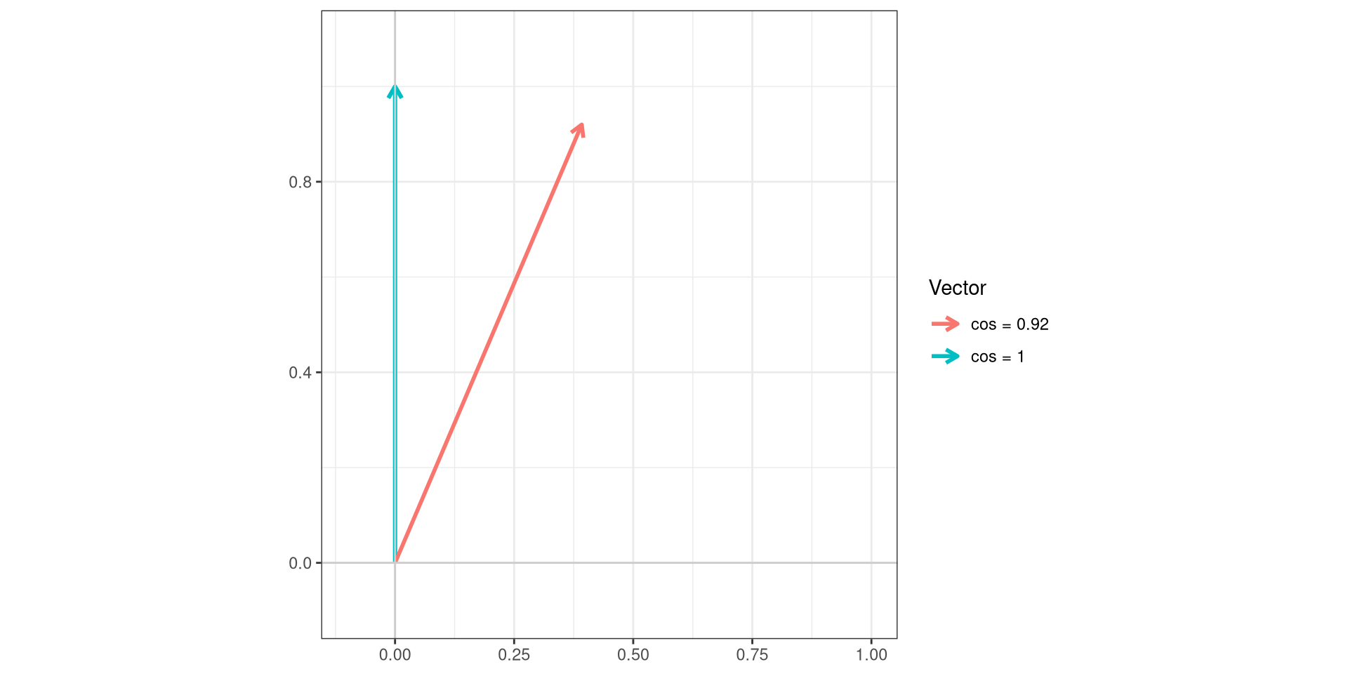
.
So in this case, the variant with residual autofluorescence if utilized as the unmixing reference signature would likely result in a fairly substantial unmixing error.
Pass
80% of the cells within our gated region are a match for the BUV395 reference signature. The other 20% of cells have residual autofluorescence contribution, which can cause a shift in the overall signature. While not abundant enough to impact the overall signature, if we wanted to prevent this scenario, we could always shift our original positive gate to the right (retaining only the brighter cells) which should reduce the overall prevalence of these two signature variants.
BUV496
.
Next up in terms of laser and peak emission detecter we have one of the most autofluorescence similar fluorophores, BUV496, conjugated in this case to CD8. Given that CD8 is a “primary” marker, and how we placed the gate, this antigen-fluorophore combination has a decent chance of being reasonably bright.
.
As was the case for the BUV395, we can start by checking the “LinearSlices_Plot”, which allows us to visualize the effect on the overall retrieved signature if we had split the region within out “positive” gate into 10% bins of increasing brightness.
.
As we might anticipate given the antigen-fluorophore pairing (alongside best practices on gate placement), there are no significant differences in the signature retrieved across the individual 10% bins.
.
We can follow up by checking the LuciernagaQC() output stored in “LuciernagaQC_Signatures”, which will group individual cell normalized signatures on the basis of shared peak and height
.
At which point, we can see only one signature is present across the board. We can go ahead and call it for this fluorophore on the other comparisons.
Pass
For BUV496, only 1 normalized fluorescent signature was present in the cells within the gated region of our reference control, so no changes are needed.
BUV563
.
One thing to keep in mind, this would be one of the single-color unmixing controls that would have been prepared with the PMA-ionomycin activated cells. The LuciernagaIntegration() wrappers default is to use the internal negative, but still worth keeping an eye on and see how it behaves compared to the previous fluorophores.
.
As was the case for the previous fluorophores, we can start by checking the “LinearSlices_Plot”, to see what the effect would have been on the signature if we had split the cells within our “positive” gate into 10% bins across.
.
We have a similar situation as what we encountered with BUV496. Lets go ahead and check the LuciernagaQC() output to see if we see any variant signatures when we group the individual cell normalized signatures by shared peak and height
.
In this case, we get back a few variant signatures, but at first glance the differences seem minimal (secondary peak “YG2” being either 20 or 30% of the primary “UV9” peak, tertiary peak “B4” either 20 or 30% of the primary “UV9” peak). These differences are likely going to be minor, driven by how Luciernaga_QC() goes about its rounding.
.
Lets still carry out the comparisons for practice for the upcoming fluorophores. We can check to see what the average would have looked like by checking the output stored under “LuciernagaQC_AmalgamatedPlot”
.
As anticipated, minimal. How were these signatures distributed across the gated cells? We can also check the output under “ProportionPlot”
.
So most cells have a secondary peak “YG2_03”, with a bit of wobble on the “B4” detector. For good measure, lets go ahead and pull the “Cosine” plot.
.
At this point, it feels unecesary to dive further since the variants all have cosine values of 1, but we can check the “Average” signature using QC_WhatsThis() for final verification.
Pass
For BUV563, we didn’t find any substantial signature variants, so our gate is likely fine as placed, and we can move on to screening the next fluorophore.
BUV615
.
Up next, we have BUV615, which is conjugated to CCR4. As far as classifying marker expression, this one is more on the chemokine side, so we should expect lower antigen density compared to what we saw for primary markers like BUV496 CD8.
.
First up, the “LinearSlices_Plot” output to check whether we would have retrieved any variant signatures had we split our “positive” gated region into 10% bins.
.
Oooh look, a new pattern! While the main signature peaks are uniform across all the percentile signatures, there is step-ladder appearance around the “V5” through “V7” peaks (as well as the “UV7” detector).
.
With these differences noted, lets check out the LuciernagaQC() output stored under “LuciernagaQC_Signatures” to see how many variant signatures we got from the grouped individual cell normalized signatures.
.
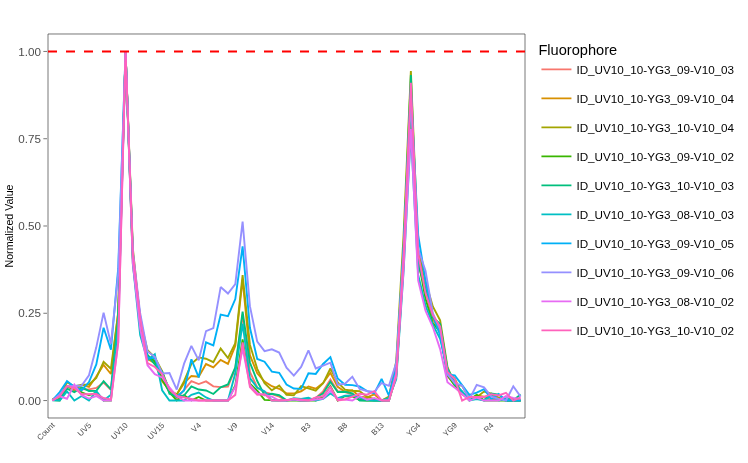
We have unlocked our first misbehaving fluorophore! We can see that all the signature variants share the same main peak (“UV10”). They also share the secondary peak (“YG3”), although this varies in height (from 80% to 100% of the main “UV10” detector). The third shared peak height is even more variable (ranging from 20 to 60% of the main “UV10” peak). All together, this may be indicative of ongoing tandem decoupling to a certain extent.
.
Additionally, the signatures that have a higher tertiary “V10” peak also exhibit higher signal in the regions that are typical of lymphocyte autofluorescence (“UV7”, “V7”, “B3”). This suggest potentially that residual autofluorescence is being leftover in the signature after background subtraction.
.
So we have signature variants, but we don’t know how prevalent they are. Lets go ahead and check under the “LuciernagaQC_AmalgamatedPlot” output to see what the median (“Average”) signature ends up at when accounting for all the cells present in the gate
.
Unlike the case we saw for BUV395 CD62L, the “Average” seems to be in the middle of the signature variants for the “V10” detector, suggesting its being influenced by the variants. For comparison, lets see what the BUV615 reference signature looks like for context.
.
So overall, the reference has a “YG3” detector closer to 0.9, a “V10” detector closer to “0.3”, so we are retrieving signature variants positioned both below and above it in regards to the “V10” detector height. We can next filter() for the average, as well as variant signatures with minimal and maxinum heights of the tertiary “V10” peak.
.
Lets pass these individually to QC_WhatsThis() and gage the difference.
.
As we may have anticipated, the signature variant “UV10_10-YG3_09-V10_06” which appeared to have the greatest amount of autofluorescence residual is the most different, coming back with a cosine value of 0.9. Lets visualize these retrieved cosines.
Code
cos_vals <- c(1, 1, 0.90)
theta <- acos(cos_vals)

df <- data.frame(
  label = paste0("cos = ", cos_vals),
  angle_deg = round(theta * 180 / pi, 1),
  x = sin(theta),
  y = cos(theta)
)

ggplot(df) +
  geom_segment(aes(x = 0, y = 0, xend = x, yend = y, color = label),
               arrow = arrow(length = unit(0.25, "cm")),
               linewidth = 1) +
  coord_fixed(xlim = c(-0.1, 1), ylim = c(-0.1, 1.1)) +
  geom_hline(yintercept = 0, color = "grey80") +
  geom_vline(xintercept = 0, color = "grey80") +
  labs(x = NULL, y = NULL, color = "Vector",
       title = NULL) +
  theme_bw()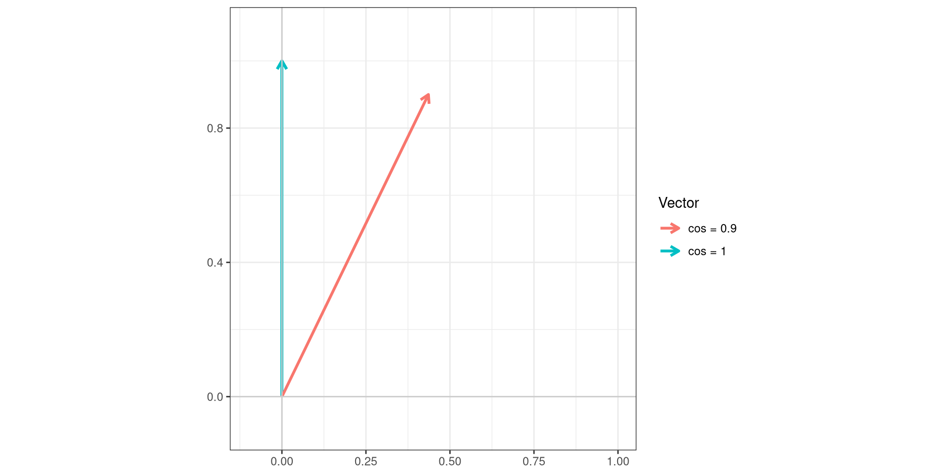
.
And finally, lets go ahead and check the “CosineSimilarityPlots” and the “ProportionPlot” before we make a decision
.
So ultimately, we have 5% of overall cells with the degraded/high-autofluorescence residual signature.
Fail
While there are still cells present that maintain BUV615 signature (and we might still rescue this control by moving the gate substantially to the right), there are clear warning signs that this particular single-color unmixing control is not in good shape, with evidence for both tandem-degradation and also residual autofluorescence contamination. Whether this is due to cell-specific degradation (like what we encountered for APC-Fire 810 during Week 12) or at the antibody vial level is something that would need to be investigated separately.
Ultimately, this was one of the antibody-fluorophore combinations for our panel that consistently caused notable unmixing issues, and it wasn’t until we switched it over to a bead single-color unmixing control that the issues cleared up, which formed the basis for our CYTO 2025 poster.
BUV661
.
Continuing on, we reach the BUV661 fluorophore, which was conjugated to Vδ2. For the original study, the Vγ9Vδ2 T cells cells were one the main cell subsets of interest.
.
While the antigen is typically expressed highly, we would normally anticipate having bright antibody-fluorophore staining. However, the Vδ2 T cell frequency can vary person to person, which means routine use in a cell single-color unmixing control requires pre-screening donors for one with high enough percentage to make acquisition sufficient bright events feasible.
.
As usual, we can check the “LinearSlices_Plot”, to see what the effect would have been on the signature if we had split the “positive” gate into 10% bins across.
.
So far, minimal differences across the percentile bins. Lets isntead check the LuciernagaQC() output to see if there are any signature variants retrieved when we group individual cell normalized signatures based on shared peak and height.
.
Two signature variants, with slightly different R1/R2 peak heights. When taking the median, where does the “Average” signature end up?
.
“Average” ends up closer to the signature with the secondary “R2_09” peak. So overall, this antigen-fluorophore combination appears to be behaving. We can wrap up by checking the cosine values.
Pass
For our BUV661, only two signature variants, both which match the reference fluorophore (with minor difference in the secondary “R2” peaks height). This minor difference may be due to difference in tandem batch conjugation or instrumental factors, but as long as we are using the same antibody on our full-stained samples as we do our single-color control, we should be okay.
BUV737
.
Up next, we have BUV737, conjugated to CXCR3. Given the ligand, the antigen-fluorophore combination may be expected to have some brightness issues similar to what we saw for BUV615 CCR4
.
Lets first take a look at the “LinearSlices_Plot”, to see if there would have been an effect on the signature if we had split the “positive” gated region across 10% bins.
.
Right off, we notice patterns similar to what we saw for BUV615 CCR4, with the main fluorophore peaks (“UV14” and “R5”) being shared across 10% bins, but uncertainty ladden step-ladder peaks for “V7”, “B3” and “UV7” detectors.
.
Lets break out LuciernagaQC() output and see what the grouped individual cell normalized signature variants are up to.
.
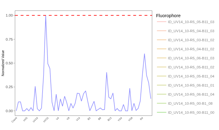
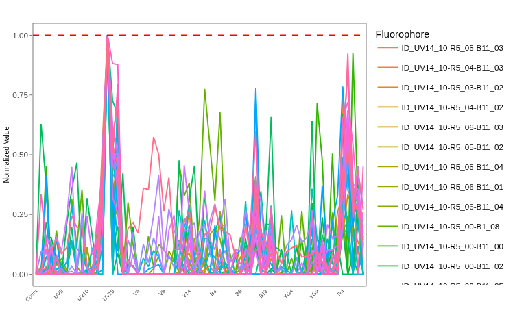
We have a fuzzy caterpillar! At this point, we are getting back way to many signature variants, many of these not well defined (likely due to insufficient number events) which contributes to the fuzzy appearance.
.
Lets see if we can at least make out the main signature appearance by checking the QC_AmalgamatedPlot() output
.
While “UV14” appears to be fairly shared, “R5” and “B11” appear to be wildly variable in terms of height. This is typical either in situations where the antibody didn’t really stain well (ending up with very dim signal, mainly consistent of non-specific staining), or major tandem degradation.
.
Let’s check “ProportionPlot” and identify the signatures that represent the majority of the cells present
.
Not particularly helpful, but if we zoom in, we can find “UV14_10-R5_06-B11_03”, “UV14_10-R5_05-B11_03”, “UV14_10-R5_04-B11_03”, “UV14_10-R5_04-B11_02” and “UV14_10-R5_03-B11_02” have more than 5% of total cells each.
.
Lets retrieve the underlying data for this plot, and select for these.
.
Lets pass these individually to QC_WhatsThis() and gage the difference.
.
Overall, for these more prevalent signatures, none match the BUV737 reference, ranging from 0.92 to 1.0 in terms of their cosine. Lets plot these angles for reference
Code
cos_vals <- c(1, 0.92, 0.97, 0.98)
theta <- acos(cos_vals)

df <- data.frame(
  label = paste0("cos = ", cos_vals),
  angle_deg = round(theta * 180 / pi, 1),
  x = sin(theta),
  y = cos(theta)
)

ggplot(df) +
  geom_segment(aes(x = 0, y = 0, xend = x, yend = y, color = label),
               arrow = arrow(length = unit(0.25, "cm")),
               linewidth = 1) +
  coord_fixed(xlim = c(-0.1, 1), ylim = c(-0.1, 1.1)) +
  geom_hline(yintercept = 0, color = "grey80") +
  geom_vline(xintercept = 0, color = "grey80") +
  labs(x = NULL, y = NULL, color = "Vector",
       title = NULL) +
  theme_bw()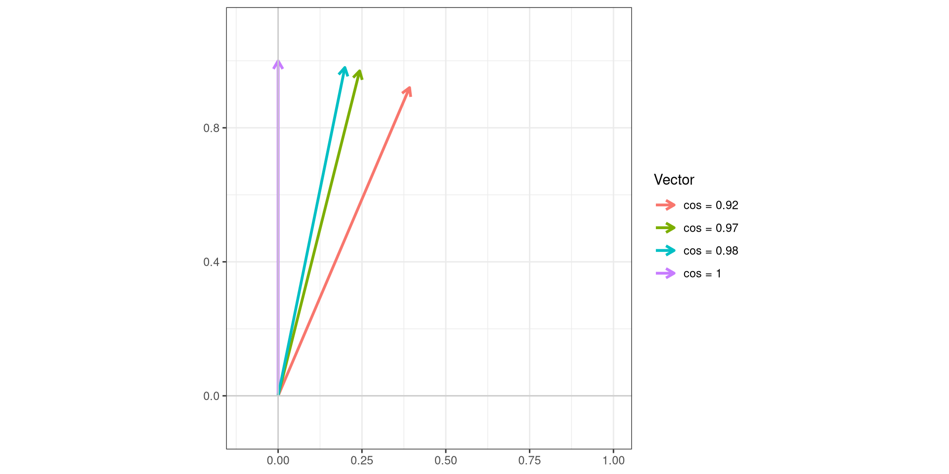
.
Ultimately, this just looks like a mess. Whether its due to a dim antigen-fluorophore combinations or tandem degradation is a story for another day.
Fail
For BUV737, this one is an immediate NO! The sheer number of variants with different heights around the secondary and tertiary peaks suggest that the tandem likely degraded.
Likewise, the step-ladders around the autofluorescence typical peaks result when the antigen-fluorophore combination is not bright enough, resulting in leftover autofluorescence residuals after background subtraction contributing significantly more to the signature shape.
This is also consistent with tandem degradation scenario, since the peaks would not be as bright as they should be to render this leftover residual insignificant compared to the overall signature.
Additionally, we can’t rule out that the antibody clone could also be a bad one, since if there was no binding to the antigen, there would no direct staining, and what we could be gating on might just be the result of non-specific noise, further adding to the dim signal/overall fuzzyness.
Ultimately, replacing this cell unmixing control for its bead single-color unmixing control is no brainer, and we should check the full-stained sample to see if there is CXCR3 staining after unmixing to determine whether the antibody clone is the root cause or not.
BUV805
.
And wrapping up our exploration of the UV laser fluorophores, lets check out the BUV805 fluorophore, which is conjugated to CD4. Given antigen density on a CD4 T cell, this should prove less complicated than the mess that was BUV737 CXCR3
.
Lets first take a look at the “LinearSlices_Plot”, to see what effect would have been on the signature if we had split the cells within our “positive” gate into 10% bins across based on brightness.
.
Pretty much no difference on the autofluorescence detectors, so very similar to what we saw for BUV496 CD8. Lets check out the LuciernagaQC() output to see what happens when we group individual cell normalized signatures based on shared peaks of similar height
.
And we end up with just 1 signature. Lets wrap this up by comparing to the reference.
Pass
For BUV805, we only retrieved 1 signature, likely due to the antigen-fluorophore combination being a bright one, and the tandem being in good shape. We are good to proceed to the next fluorophore!
Violet
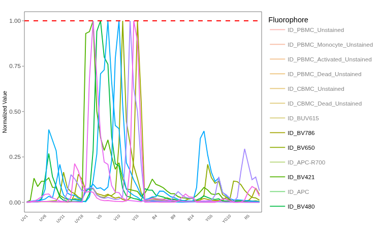
.
Due to the sheer number of plotly ggplotly() interactive plots that the website would need to load if we had visualized all the LuciernagaIntegration() plots for the 29-fluorophore panel in one go, we have broken the exploration of the fluorophore outputs by laser. The walk-through of the “Violet” fluorophores has been migrated here.
Blue
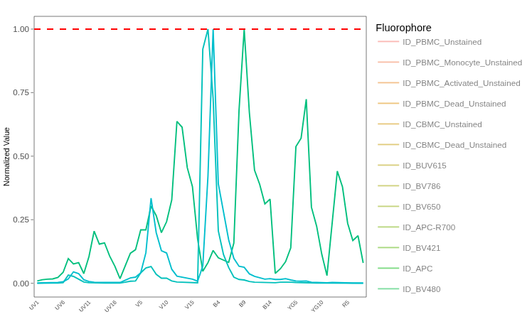
.
Due to the sheer number of plotly ggplotly() interactive plots that the website would need to load if we had visualized all the LuciernagaIntegration() plots for the 29-fluorophore panel in one go, we have broken the exploration of the fluorophore outputs by laser. The walk-through of the “Blue” fluorophores has been migrated here.
Yellow-Green
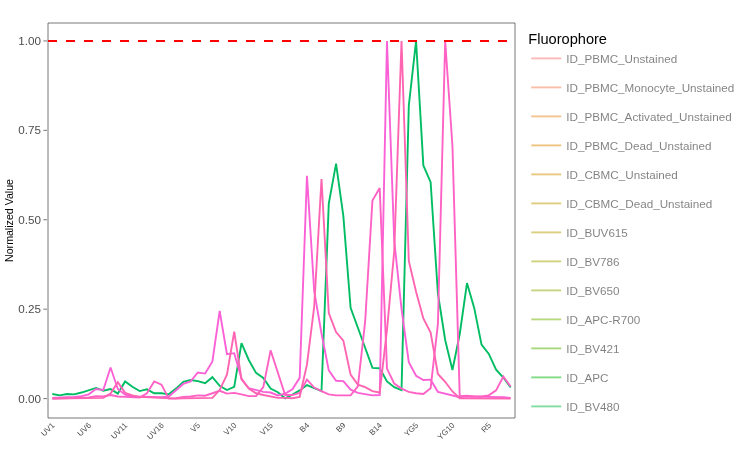
.
Due to the sheer number of plotly ggplotly() interactive plots that the website would need to load if we had visualized all the LuciernagaIntegration() plots for the 29-fluorophore panel in one go, we have broken the exploration of the fluorophore outputs by laser. The walk-through of the “Yellow-Green” fluorophores has been migrated here.
Red
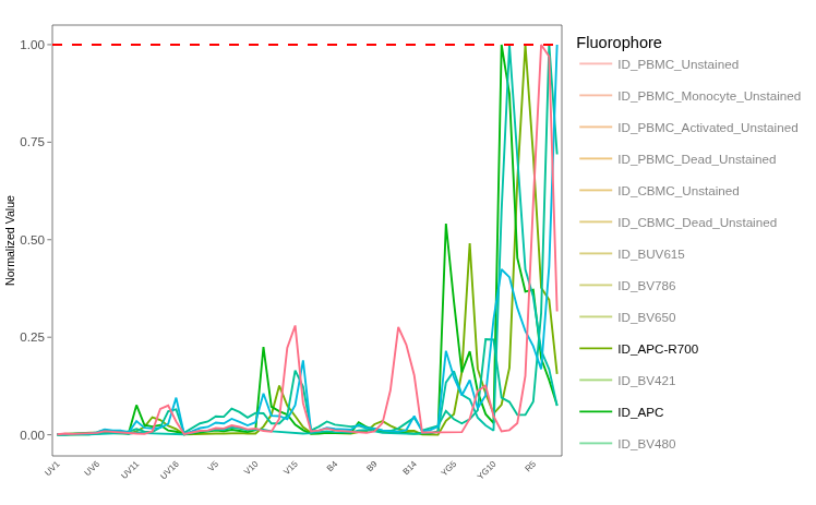
.
Due to the sheer number of plotly ggplotly() interactive plots that the website would need to load if we had visualized all the LuciernagaIntegration() plots for the 29-fluorophore panel in one go, we have broken the exploration of the fluorophore outputs by laser. The walk-through of the “Red” fluorophores has been migrated here.
Autofluorescence
.
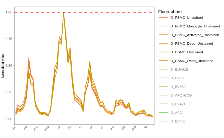
Due to the sheer number of plotly ggplotly() interactive plots that the website would need to load if we had visualized all the LuciernagaIntegration() plots for the 29-fluorophore panel in one go, we have broken the exploration of the fluorophore outputs by laser. The walk-through of the “Unstained” signatures has been migrated here.
Take Away
.
In this walk-through (and its subsetted “Laser” chapters), we have systematically worked our way through the unmixing controls (both single-color and unstained) for this 29-color panel. Overall, most of the fluorophores were in good shape, only returning a single signature for cells within our gated region, or with signature variants that were highly similar and not likely to cause much trouble at the time of unmixing.
.
And then, we also encountered 6 problematic cell single-color unmixing controls. These included
- BUV615
- BUV737
- BV421
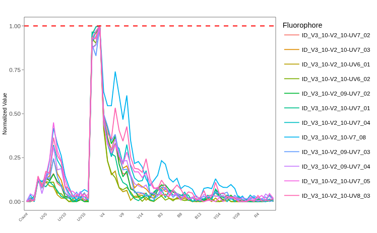
- PerCP-Cy5.5 (not a proper fail, but a caution)
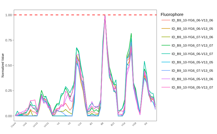
- PE-Cy5
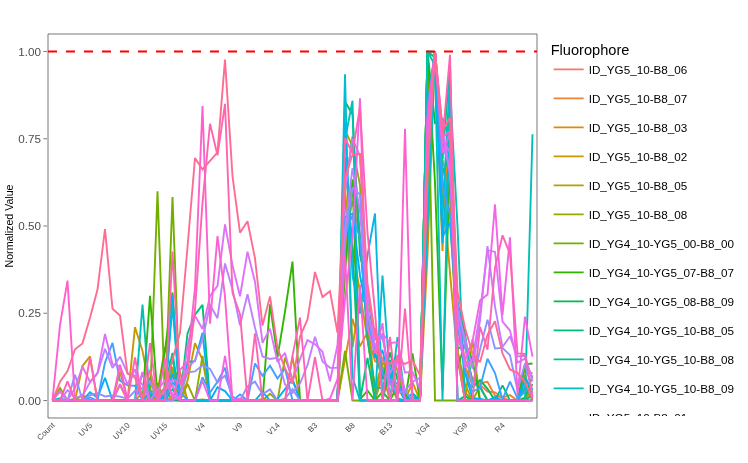
- APC-Fire 810
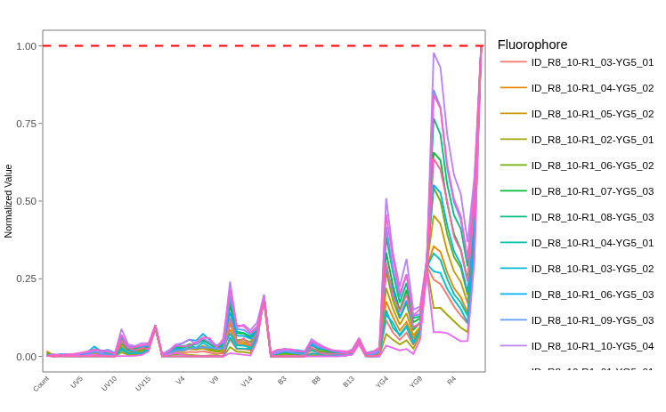
.
While differing in their extent, BUV737, PE-Cy5 and APC-Fire 810 are in the worst shape, and would likely cause issues with the unmixing of the full-stained samples if they were included within the unmixing matrix.
.
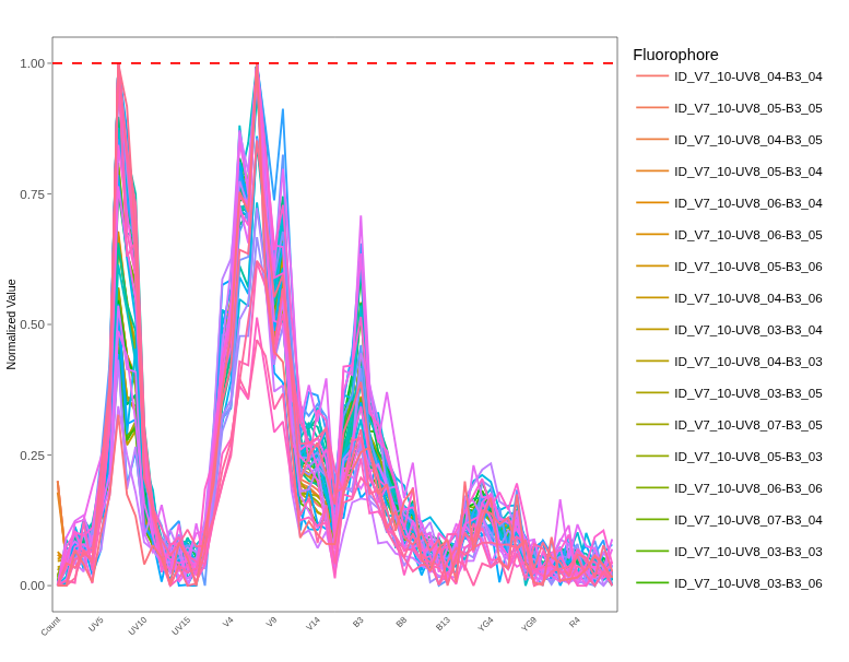
Likewise, we looked at unstained samples and characterized the autofluorescence variation that is present within. Main things we noticed were shift in secondary peak usage for cord blood vs peripheral blood mononuclear cells, and some interesting variation in the height of the secondary “UV7” detector that ties into how similar the signature compares to our autofluorescence-similar fluorophores.
- INF052 Ctrl (CBMC)
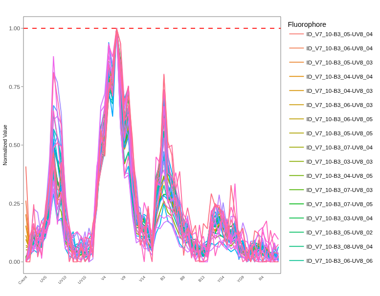
- ND006 Ctrl (PBMC)
.
We will circle back to these bad unmixing control signatures during Week 15 and evaluate what kind of unmixing errors they would generate compared to full-stained samples that had been unmixed with more representative fluorophore signatures. Until then, have fun looking at your own single-color unmixing controls, and make sure to share any interesting tandem-degradation finds on the Discussions Page
Additional Resources
Luciernaga Vignette - Reference Library
Luciernaga Vignette - Fluorescent Signatures