07 - Applying Transformations
2026-03-24

![]()
![]()
Background
.
Week 7: For this seventh session, we take a closer look at the raw values of the data within our .fcs files, and explore the various ways to transform (ie. scale) flow cytometry data in R to better visualize “positive” and “negative populations”.
.
There exist several commonly used transformations for Flow Cytometry data. Similarly, for Mass Cytometry data, the arsinh transformation is the most frequently applied.
.
Regardless of method, the goal remains to rescale the data in a way that allows for better interpretation. A misapplied transformation can be dangerous for an analysis, so don’t just accept the default. Always ensure that what your transformed data visually makes sense. Similarly, this approach is shared in many of the exploratory data analsyis approaches we will encounter later on during the course.
.
Additionally, due to near perfect timing, Felix Marsh-Wakefield did a good overview of transformation for CytoBites YouTube channel earlier this week that is worth checking out.
Walk Through
Housekeeping
As we do every week, on GitHub, sync your forked version of the CytometryInR course to bring in the most recent updates. Then within Positron, pull in those changes to your local computer.
For YouTube walkthrough of this process, click here
After setting up a “Week07” project folder, copy over the contents of “course/06_Visualizing/data” to that folder. This will hopefully prevent merge issues next week when attempting to pull in new course material. Once you have your new project folder organized, remember to commit and push your changes to GitHub to maintain remote version control.
If you encounter issues syncing due to the Take-Home Problem merge conflict, see this walkthrough. The updated homework submission protocol can be found here
Load Libraries
.
This week, we will extensively be using the flowWorkspace package, as we learn how to build out our own GatingSet objects to include transformations. As we do so, we will need to visualize our underlying data, to ensure that the transformartions applied were correct for our datasets. Consequently, we will be using the ggcyto package extensively throughout the day. Therefore, it makes sense to go ahead and attach both packages to our local environment from the start.
Separating SFC and MC fcs files
.
We will be using two cytometry datasets this week. For the Spectral Flow Cytometry dataset, we will be re-using the 6 unmixed .fcs file first shared during Week 05. This time around, rather than bring them from a FlowJo.wsp into a GatingSet via the CytoML package, we will be building the GatingSet from scratch using the flowWorkspace package. These .fcs file names share the “2025” portion in the name, which we will use to filter them from the list.files() vector list.
.
For the Mass Cytometry dataset, we will be using 3 .fcs files that I retrieved from ImmPort for the Study SDY2739 (Clinical Immunity to Malaria Involves Epigenetic Reprogramming of Innate Immune Cells). The .fcs file names for these files share the “G1_2” portion in the name, which we will use to filter them from the list.files() vector list.
#StorageLocation <- file.path("course", "07_Transformations", "data") # When interactively writing the code

StorageLocation <- file.path("data") #When Quarto Rendering

fcs_files <- list.files(StorageLocation, ".fcs", full.names=TRUE)
SFC_files <- fcs_files[stringr::str_detect(fcs_files, "2025")]
MC_files <- fcs_files[stringr::str_detect(fcs_files, "G1_2")]
.
Lets start by working with the SFC dataset. First off, let’s double check that we have just the SFC files (as flowWorkspace will throw an error if the .fcs files passed contain different number of fluorophore/metal columns)
.
Circling back to where we left off during Week 05, we will pass these file path locations to load_cytoset_from_fcs() to load them into a GatingSet object.
Metadata
.
One worthwile thing when first starting is to check the metadata for the GatingSet, using the pData() function.
                                                                   name
2025_07_26_AB_02_INF052_00_Ctrl.fcs 2025_07_26_AB_02_INF052_00_Ctrl.fcs
2025_07_26_AB_02_INF052_00_SEB.fcs   2025_07_26_AB_02_INF052_00_SEB.fcs
2025_07_26_AB_02_INF100_00_Ctrl.fcs 2025_07_26_AB_02_INF100_00_Ctrl.fcs
2025_07_26_AB_02_INF100_00_SEB.fcs   2025_07_26_AB_02_INF100_00_SEB.fcs
2025_07_26_AB_02_INF179_00_Ctrl.fcs 2025_07_26_AB_02_INF179_00_Ctrl.fcs
2025_07_26_AB_02_INF179_00_SEB.fcs   2025_07_26_AB_02_INF179_00_SEB.fcs
.
In the current form, the metadata is kinda empty, only containing rownames and the name column. However, we can notice that within the existing names, we have some useful information present between the underscores that we might be able to extract out and append as additional metadata colums.
.
Lets first off retrieve the metadata by assigning to its own object/variable
.
As you can see, it is just a data.frame style object that we have encountered in the past. We can therefore use dplyr package functions to help us tidy the metadata to extract the additional information that we may need in the future. Let’s go ahead and load in dplyr
.
And then create a new column for Condition so that we can better evaluate how the various extraction functions work, and also not risk messing up the underlying data while testing out how to use several new functions.
RegEx
.
Glancing at the current names, we can notice that if we wanted to extract the Condition (Ctrl, PPD, SEB), we would need to remove all character values up the final underscore (_), and before the “.fcs”.
.
Within base R, two functions, sub() and gsub() are most frequently encountered when attempting to extract out a particular pattern. These rely on providing a regular expression (RegEx) pattern to match, and a replacement value to swap in its place (which can be left empty by providing a ““).
.
Consequently, if we were using sub(), our first step to replace everything up through the last underscore would be the RegEx expression “.*_”
.
And we could follow up by matching the “.fcs” pattern and leaving the replacement value as “” as well.
Tip
Please be advised, even with years of practice, I still will struggle to remember the proper RegEx syntax code to extract out a pattern from a long complicated character string. This is one use case where having a LLM provide a narrowly focused answer can be quite useful. Prompt example:
“I am working in R, using sub(), I want to keep everything after the last _ : 2025_07_26_AB_02_INF052_00_Ctrl.fcs”
.
In addition to sub() and gsub() in base R, we can also achieve a similar outcome using the stringr package from the tidyverse, using the str_extract() function (after investigating the correct RegEx style syntax). To interpret this RegEx-inspired hieroglyphic, note that “^” is used for the start of a string, and “$” for the end of the string. So we are extracting the pattern after the underscore “^_“, but keeping the contents before the final .fcs
.
So, wrapping it all together, we could write the following to create a Condition column
                                                                   name
2025_07_26_AB_02_INF052_00_Ctrl.fcs 2025_07_26_AB_02_INF052_00_Ctrl.fcs
2025_07_26_AB_02_INF052_00_SEB.fcs   2025_07_26_AB_02_INF052_00_SEB.fcs
2025_07_26_AB_02_INF100_00_Ctrl.fcs 2025_07_26_AB_02_INF100_00_Ctrl.fcs
2025_07_26_AB_02_INF100_00_SEB.fcs   2025_07_26_AB_02_INF100_00_SEB.fcs
2025_07_26_AB_02_INF179_00_Ctrl.fcs 2025_07_26_AB_02_INF179_00_Ctrl.fcs
2025_07_26_AB_02_INF179_00_SEB.fcs   2025_07_26_AB_02_INF179_00_SEB.fcs
                                    Condition
2025_07_26_AB_02_INF052_00_Ctrl.fcs      Ctrl
2025_07_26_AB_02_INF052_00_SEB.fcs        SEB
2025_07_26_AB_02_INF100_00_Ctrl.fcs      Ctrl
2025_07_26_AB_02_INF100_00_SEB.fcs        SEB
2025_07_26_AB_02_INF179_00_Ctrl.fcs      Ctrl
2025_07_26_AB_02_INF179_00_SEB.fcs        SEB
.
Fortunately, extracting an actual pattern is a bit simpler, so we can similarly grab the specimen ID number.
                                    Condition Specimen
2025_07_26_AB_02_INF052_00_Ctrl.fcs      Ctrl   INF052
2025_07_26_AB_02_INF052_00_SEB.fcs        SEB   INF052
2025_07_26_AB_02_INF100_00_Ctrl.fcs      Ctrl   INF100
2025_07_26_AB_02_INF100_00_SEB.fcs        SEB   INF100
2025_07_26_AB_02_INF179_00_Ctrl.fcs      Ctrl   INF179
2025_07_26_AB_02_INF179_00_SEB.fcs        SEB   INF179
Updating Metadata
.
When binding columns from two separate data.frame objects in R, we can use the cbind() base R function.
                                                                   name
2025_07_26_AB_02_INF052_00_Ctrl.fcs 2025_07_26_AB_02_INF052_00_Ctrl.fcs
2025_07_26_AB_02_INF052_00_SEB.fcs   2025_07_26_AB_02_INF052_00_SEB.fcs
2025_07_26_AB_02_INF100_00_Ctrl.fcs 2025_07_26_AB_02_INF100_00_Ctrl.fcs
2025_07_26_AB_02_INF100_00_SEB.fcs   2025_07_26_AB_02_INF100_00_SEB.fcs
2025_07_26_AB_02_INF179_00_Ctrl.fcs 2025_07_26_AB_02_INF179_00_Ctrl.fcs
2025_07_26_AB_02_INF179_00_SEB.fcs   2025_07_26_AB_02_INF179_00_SEB.fcs
                                    Condition Specimen
2025_07_26_AB_02_INF052_00_Ctrl.fcs      Ctrl   INF052
2025_07_26_AB_02_INF052_00_SEB.fcs        SEB   INF052
2025_07_26_AB_02_INF100_00_Ctrl.fcs      Ctrl   INF100
2025_07_26_AB_02_INF100_00_SEB.fcs        SEB   INF100
2025_07_26_AB_02_INF179_00_Ctrl.fcs      Ctrl   INF179
2025_07_26_AB_02_INF179_00_SEB.fcs        SEB   INF179
.
Which we can then use to overwrite the existing metadata present for the GatingSet.
                                                                   name
2025_07_26_AB_02_INF052_00_Ctrl.fcs 2025_07_26_AB_02_INF052_00_Ctrl.fcs
2025_07_26_AB_02_INF052_00_SEB.fcs   2025_07_26_AB_02_INF052_00_SEB.fcs
2025_07_26_AB_02_INF100_00_Ctrl.fcs 2025_07_26_AB_02_INF100_00_Ctrl.fcs
2025_07_26_AB_02_INF100_00_SEB.fcs   2025_07_26_AB_02_INF100_00_SEB.fcs
2025_07_26_AB_02_INF179_00_Ctrl.fcs 2025_07_26_AB_02_INF179_00_Ctrl.fcs
2025_07_26_AB_02_INF179_00_SEB.fcs   2025_07_26_AB_02_INF179_00_SEB.fcs
                                    Specimen Condition
2025_07_26_AB_02_INF052_00_Ctrl.fcs   INF052      Ctrl
2025_07_26_AB_02_INF052_00_SEB.fcs    INF052       SEB
2025_07_26_AB_02_INF100_00_Ctrl.fcs   INF100      Ctrl
2025_07_26_AB_02_INF100_00_SEB.fcs    INF100       SEB
2025_07_26_AB_02_INF179_00_Ctrl.fcs   INF179      Ctrl
2025_07_26_AB_02_INF179_00_SEB.fcs    INF179       SEB
.
Which we can use to subset the GatingSet in the future
                                                                 name Specimen
2025_07_26_AB_02_INF052_00_SEB.fcs 2025_07_26_AB_02_INF052_00_SEB.fcs   INF052
2025_07_26_AB_02_INF100_00_SEB.fcs 2025_07_26_AB_02_INF100_00_SEB.fcs   INF100
2025_07_26_AB_02_INF179_00_SEB.fcs 2025_07_26_AB_02_INF179_00_SEB.fcs   INF179
                                   Condition
2025_07_26_AB_02_INF052_00_SEB.fcs       SEB
2025_07_26_AB_02_INF100_00_SEB.fcs       SEB
2025_07_26_AB_02_INF179_00_SEB.fcs       SEB
SFC
.
Having emerged from the metadata, let’s return to focusing on our SFC dataset.
colnames
.
When working with .fcs files that we have not worked with recently, it is often good to go ahead and check to see what fluorophores/markers are present at the start. This is also useful as different cytometer platforms have slightly different naming conventions. We can use colnames()
 [1] "Time"              "SSC-W"             "SSC-H"
 [4] "SSC-A"             "FSC-W"             "FSC-H"
 [7] "FSC-A"             "SSC-B-W"           "SSC-B-H"
[10] "SSC-B-A"           "BUV395-A"          "BUV563-A"
[13] "BUV615-A"          "BUV661-A"          "BUV737-A"
[16] "BUV805-A"          "Pacific Blue-A"    "BV480-A"
[19] "BV570-A"           "BV605-A"           "BV650-A"
[22] "BV711-A"           "BV750-A"           "BV786-A"
[25] "Alexa Fluor 488-A" "Spark Blue 550-A"  "Spark Blue 574-A"
[28] "RB613-A"           "RB705-A"           "RB780-A"
[31] "PE-A"              "PE-Dazzle594-A"    "PE-Cy5-A"
[34] "PE-Fire 700-A"     "PE-Fire 744-A"     "PE-Vio770-A"
[37] "APC-A"             "Alexa Fluor 647-A" "APC-R700-A"
[40] "Zombie NIR-A"      "APC-Fire 750-A"    "APC-Fire 810-A"
[43] "AF-A"
.
As we can see from the output, most of the fluorophores have an “-A” appended to the end, although the FSC and SSC parameters feature area, height and width (“-A”, “-H”, “-W”) respectively.
markernames
         BUV395-A          BUV563-A          BUV615-A          BUV661-A
          "CD62L"            "CD69"            "CCR4"             "Vd2"
         BUV737-A          BUV805-A    Pacific Blue-A           BV480-A
           "CD38"             "CD4"            "Dump"           "CD161"
          BV570-A           BV605-A           BV650-A           BV711-A
           "CD16"          "CD45RA"             "CD8"           "Va7.2"
          BV750-A           BV786-A Alexa Fluor 488-A  Spark Blue 550-A
           "IFNg"            "CCR6"           "FoxP3"             "CD3"
 Spark Blue 574-A           RB613-A           RB705-A           RB780-A
           "CD45"             "PD1"            "CD26"           "CXCR5"
             PE-A    PE-Dazzle594-A          PE-Cy5-A     PE-Fire 700-A
           "ICOS"            "TNFa"           "CXCR3"           "CD127"
    PE-Fire 744-A       PE-Vio770-A             APC-A Alexa Fluor 647-A
           "CD25"          "HLA-DR"            "CD39"            "IL-2"
       APC-R700-A      Zombie NIR-A    APC-Fire 750-A    APC-Fire 810-A
         "CD107a"       "Viability"            "CD27"            "CCR7"
ggcyto
.
At this point, we can then use what we have learned about the ggcyto package to make sure that the FSC x SSC plotting is working correctly.

.
Please note, that for ggcyto it’s just one set of [] after the GatingSet name to subset for plotting.
.
By contrast, accidentally including two sets of [] would result in accidentally breaking into the S4 internals, and getting back a GatingHierarchy.
Untransformed Data
.
Let’s go ahead and plot a couple of the fluorophores, to see what untransformed data in R looks like
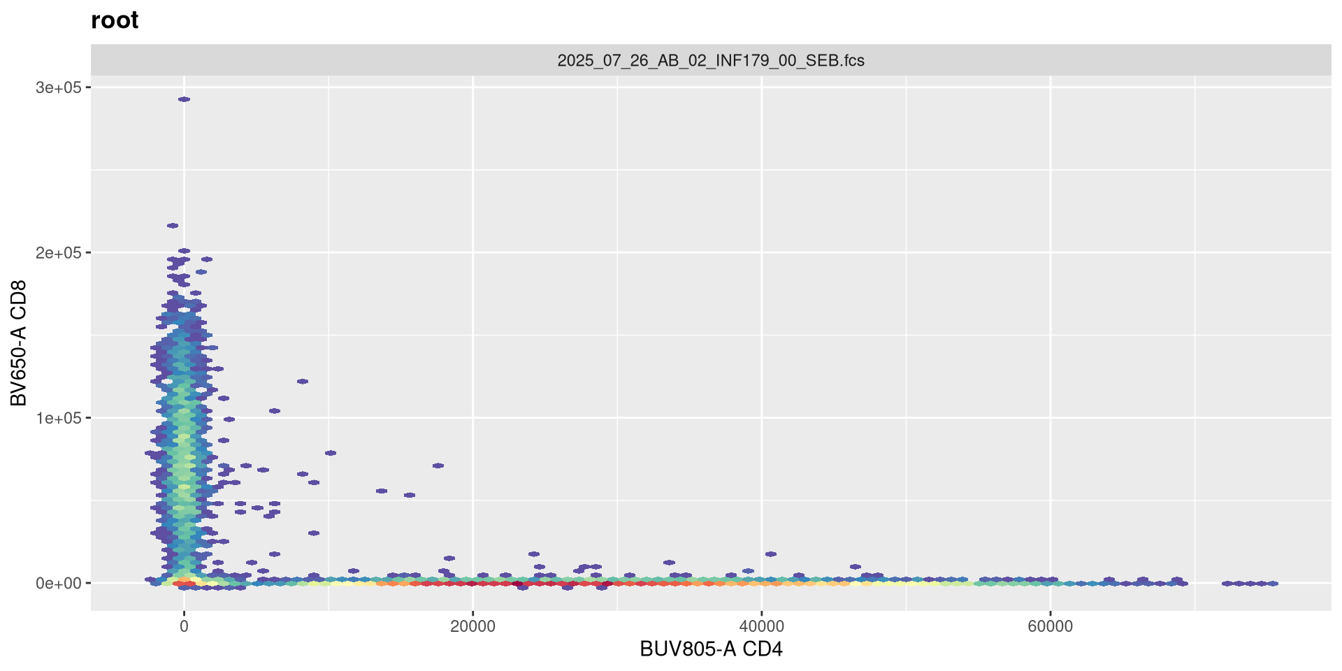
.
As we can see, the scale currently appears linear, with a wide stretch of positive values for both CD4 and CD8 T cells. By contrast, you may remember the transformed version brought for this same .fcs file brought in from FlowJo via CytoML resembled the following
![]()
.
If we use the gh_get_transformations function, we can see that there are currently no transformations applied to the GatingSet.
Transformers
.
flowWorkspace provides several default transforms (with the option to create your own). The functions in question return transformer objects, which are list that collect the required information for the transformations that are subsequently applied.
List of 9
 $ name        : chr "logicle"
 $ transform   :function (x)
 $ inverse     :function (x)
 $ d_transform : NULL
 $ d_inverse   : NULL
 $ breaks      :function (x)
 $ minor_breaks:function (b, limits, n)
 $ format      :function (x)
 $ domain      : num [1:2] -Inf Inf
- attr(*, "class")= chr "transform"List of 9
$ name : chr "flowJo_biexp"
$ transform :function (x, deriv = 0)
..- attr(*, "type")= chr "biexp"
..- attr(*, "parameters")=List of 5
.. ..$ channelRange: int 4096
.. ..$ maxValue : num 262144
.. ..$ neg : num 0
.. ..$ pos : num 4.5
.. ..$ widthBasis : num -10
$ inverse :function (x, deriv = 0)
..- attr(*, "type")= chr "biexp"
..- attr(*, "parameters")=List of 5
.. ..$ channelRange: int 4096
.. ..$ maxValue : num 262144
.. ..$ neg : num 0
.. ..$ pos : num 4.5
.. ..$ widthBasis : num -10
$ d_transform : NULL
$ d_inverse : NULL
$ breaks :function (x)
$ minor_breaks:function (b, limits, n)
$ format :function (x)
$ domain : num [1:2] -Inf Inf
- attr(*, "class")= chr "transform"List of 9
$ name : chr "flowJo_fasinh"
$ transform :function (x)
$ inverse :function (x)
$ d_transform : NULL
$ d_inverse : NULL
$ breaks :function (x)
$ minor_breaks:function (b, limits, n)
$ format :function (x)
$ domain : num [1:2] -Inf Inf
- attr(*, "class")= chr "transform"List of 9
$ name : chr "asinhtGml2"
$ transform :function (x)
$ inverse :function (x)
$ d_transform : NULL
$ d_inverse : NULL
$ breaks :function (x)
$ minor_breaks:function (b, limits, n)
$ format :function (x)
$ domain : num [1:2] -Inf Inf
- attr(*, "class")= chr "transform".
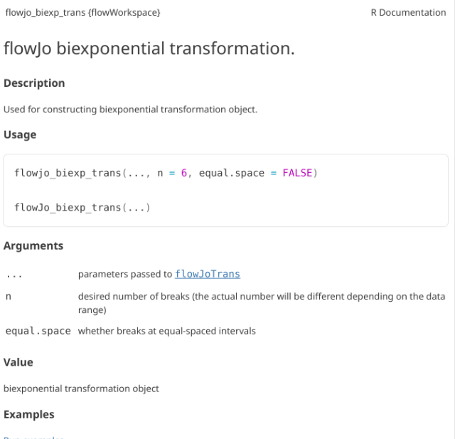
As always, it can be worthwhile to first check the help documentation, to investigate the various arguments that can be used within the setup.
Column names to be transformed
.
While having the transformation parameters is one component, the other is the fluorophores that are to be transformed. Recalling the colnames() function, we can see we have the following fluorophores for this panel.
 [1] "Time"              "SSC-W"             "SSC-H"
 [4] "SSC-A"             "FSC-W"             "FSC-H"
 [7] "FSC-A"             "SSC-B-W"           "SSC-B-H"
[10] "SSC-B-A"           "BUV395-A"          "BUV563-A"
[13] "BUV615-A"          "BUV661-A"          "BUV737-A"
[16] "BUV805-A"          "Pacific Blue-A"    "BV480-A"
[19] "BV570-A"           "BV605-A"           "BV650-A"
[22] "BV711-A"           "BV750-A"           "BV786-A"
[25] "Alexa Fluor 488-A" "Spark Blue 550-A"  "Spark Blue 574-A"
[28] "RB613-A"           "RB705-A"           "RB780-A"
[31] "PE-A"              "PE-Dazzle594-A"    "PE-Cy5-A"
[34] "PE-Fire 700-A"     "PE-Fire 744-A"     "PE-Vio770-A"
[37] "APC-A"             "Alexa Fluor 647-A" "APC-R700-A"
[40] "Zombie NIR-A"      "APC-Fire 750-A"    "APC-Fire 810-A"
[43] "AF-A"
.
We will only need to apply transformations to fluorophores, not to FSC, SSC or Time parameters. We will therefore need to remove these from the list. One way would be to use [] index method, combining a ! and stringr str_detect() to remove for values that would be shared by those parameters
 [1] "BUV395-A"          "BUV563-A"          "BUV615-A"
 [4] "BUV661-A"          "BUV737-A"          "BUV805-A"
 [7] "Pacific Blue-A"    "BV480-A"           "BV570-A"
[10] "BV605-A"           "BV650-A"           "BV711-A"
[13] "BV750-A"           "BV786-A"           "Alexa Fluor 488-A"
[16] "Spark Blue 550-A"  "Spark Blue 574-A"  "RB613-A"
[19] "RB705-A"           "RB780-A"           "PE-A"
[22] "PE-Dazzle594-A"    "PE-Cy5-A"          "PE-Fire 700-A"
[25] "PE-Fire 744-A"     "PE-Vio770-A"       "APC-A"
[28] "Alexa Fluor 647-A" "APC-R700-A"        "Zombie NIR-A"
[31] "APC-Fire 750-A"    "APC-Fire 810-A"    "AF-A"
transformerList
.
Now that we have the fluorophore columns identified, using the transformerList() function we can combine them with the Transformer object we previously created.
$`BUV395-A`
Transformer: flowJo_biexp [-Inf, Inf]

$`BUV563-A`
Transformer: flowJo_biexp [-Inf, Inf]

$`BUV615-A`
Transformer: flowJo_biexp [-Inf, Inf]

$`BUV661-A`
Transformer: flowJo_biexp [-Inf, Inf]

$`BUV737-A`
Transformer: flowJo_biexp [-Inf, Inf]

$`BUV805-A`
Transformer: flowJo_biexp [-Inf, Inf]

$`Pacific Blue-A`
Transformer: flowJo_biexp [-Inf, Inf]

$`BV480-A`
Transformer: flowJo_biexp [-Inf, Inf]

$`BV570-A`
Transformer: flowJo_biexp [-Inf, Inf]

$`BV605-A`
Transformer: flowJo_biexp [-Inf, Inf]

$`BV650-A`
Transformer: flowJo_biexp [-Inf, Inf]

$`BV711-A`
Transformer: flowJo_biexp [-Inf, Inf]

$`BV750-A`
Transformer: flowJo_biexp [-Inf, Inf]

$`BV786-A`
Transformer: flowJo_biexp [-Inf, Inf]

$`Alexa Fluor 488-A`
Transformer: flowJo_biexp [-Inf, Inf]

$`Spark Blue 550-A`
Transformer: flowJo_biexp [-Inf, Inf]

$`Spark Blue 574-A`
Transformer: flowJo_biexp [-Inf, Inf]

$`RB613-A`
Transformer: flowJo_biexp [-Inf, Inf]

$`RB705-A`
Transformer: flowJo_biexp [-Inf, Inf]

$`RB780-A`
Transformer: flowJo_biexp [-Inf, Inf]

$`PE-A`
Transformer: flowJo_biexp [-Inf, Inf]

$`PE-Dazzle594-A`
Transformer: flowJo_biexp [-Inf, Inf]

$`PE-Cy5-A`
Transformer: flowJo_biexp [-Inf, Inf]

$`PE-Fire 700-A`
Transformer: flowJo_biexp [-Inf, Inf]

$`PE-Fire 744-A`
Transformer: flowJo_biexp [-Inf, Inf]

$`PE-Vio770-A`
Transformer: flowJo_biexp [-Inf, Inf]

$`APC-A`
Transformer: flowJo_biexp [-Inf, Inf]

$`Alexa Fluor 647-A`
Transformer: flowJo_biexp [-Inf, Inf]

$`APC-R700-A`
Transformer: flowJo_biexp [-Inf, Inf]

$`Zombie NIR-A`
Transformer: flowJo_biexp [-Inf, Inf]

$`APC-Fire 750-A`
Transformer: flowJo_biexp [-Inf, Inf]

$`APC-Fire 810-A`
Transformer: flowJo_biexp [-Inf, Inf]

$`AF-A`
Transformer: flowJo_biexp [-Inf, Inf]

attr(,"class")
[1] "transformerList" "list" List of 3
$ BUV395-A:List of 9
..$ name : chr "flowJo_biexp"
..$ transform :function (x, deriv = 0)
.. ..- attr(*, "type")= chr "biexp"
.. ..- attr(*, "parameters")=List of 5
.. .. ..$ channelRange: int 4096
.. .. ..$ maxValue : num 262144
.. .. ..$ neg : num 0
.. .. ..$ pos : num 4.5
.. .. ..$ widthBasis : num -10
..$ inverse :function (x, deriv = 0)
.. ..- attr(*, "type")= chr "biexp"
.. ..- attr(*, "parameters")=List of 5
.. .. ..$ channelRange: int 4096
.. .. ..$ maxValue : num 262144
.. .. ..$ neg : num 0
.. .. ..$ pos : num 4.5
.. .. ..$ widthBasis : num -10
..$ d_transform : NULL
..$ d_inverse : NULL
..$ breaks :function (x)
..$ minor_breaks:function (b, limits, n)
..$ format :function (x)
..$ domain : num [1:2] -Inf Inf
..- attr(*, "class")= chr "transform"
$ BUV563-A:List of 9
..$ name : chr "flowJo_biexp"
..$ transform :function (x, deriv = 0)
.. ..- attr(*, "type")= chr "biexp"
.. ..- attr(*, "parameters")=List of 5
.. .. ..$ channelRange: int 4096
.. .. ..$ maxValue : num 262144
.. .. ..$ neg : num 0
.. .. ..$ pos : num 4.5
.. .. ..$ widthBasis : num -10
..$ inverse :function (x, deriv = 0)
.. ..- attr(*, "type")= chr "biexp"
.. ..- attr(*, "parameters")=List of 5
.. .. ..$ channelRange: int 4096
.. .. ..$ maxValue : num 262144
.. .. ..$ neg : num 0
.. .. ..$ pos : num 4.5
.. .. ..$ widthBasis : num -10
..$ d_transform : NULL
..$ d_inverse : NULL
..$ breaks :function (x)
..$ minor_breaks:function (b, limits, n)
..$ format :function (x)
..$ domain : num [1:2] -Inf Inf
..- attr(*, "class")= chr "transform"
$ BUV615-A:List of 9
..$ name : chr "flowJo_biexp"
..$ transform :function (x, deriv = 0)
.. ..- attr(*, "type")= chr "biexp"
.. ..- attr(*, "parameters")=List of 5
.. .. ..$ channelRange: int 4096
.. .. ..$ maxValue : num 262144
.. .. ..$ neg : num 0
.. .. ..$ pos : num 4.5
.. .. ..$ widthBasis : num -10
..$ inverse :function (x, deriv = 0)
.. ..- attr(*, "type")= chr "biexp"
.. ..- attr(*, "parameters")=List of 5
.. .. ..$ channelRange: int 4096
.. .. ..$ maxValue : num 262144
.. .. ..$ neg : num 0
.. .. ..$ pos : num 4.5
.. .. ..$ widthBasis : num -10
..$ d_transform : NULL
..$ d_inverse : NULL
..$ breaks :function (x)
..$ minor_breaks:function (b, limits, n)
..$ format :function (x)
..$ domain : num [1:2] -Inf Inf
..- attr(*, "class")= chr "transform"List of 9
$ name : chr "flowJo_biexp"
$ transform :function (x, deriv = 0)
..- attr(*, "type")= chr "biexp"
..- attr(*, "parameters")=List of 5
.. ..$ channelRange: int 4096
.. ..$ maxValue : num 262144
.. ..$ neg : num 0
.. ..$ pos : num 4.5
.. ..$ widthBasis : num -10
$ inverse :function (x, deriv = 0)
..- attr(*, "type")= chr "biexp"
..- attr(*, "parameters")=List of 5
.. ..$ channelRange: int 4096
.. ..$ maxValue : num 262144
.. ..$ neg : num 0
.. ..$ pos : num 4.5
.. ..$ widthBasis : num -10
$ d_transform : NULL
$ d_inverse : NULL
$ breaks :function (x)
$ minor_breaks:function (b, limits, n)
$ format :function (x)
$ domain : num [1:2] -Inf Inf
- attr(*, "class")= chr "transform".
As you can notice, for each of the fluorophores we specified, the transformer object with the desired parameters has now been added as its own list entry.
.
The final step is to then apply it to the GatingSet
.
If we now replot without having provided any arguments, we get the following:

.
As we can see, applying a default transformation to a random .fcs file is not quite the way to go. We will need to look up some of the specific parameter arguments that need to be provided. Going back to our transformer function
.
In this case, the help documentation doesn’t provide much immediately. Part of this is that flowjo_biexp_trans() appears to be a wrapper function, which passes arguments on to the flowJoTrans() function. If we look this one up
.
Under usage, we can see what the default options and arguments are.
Transformation Arguments
.
Lets evaluate what effect changing each of these arguments in has on visualizing our .fcs file. Our current visual is
SFC_cytoset <- load_cytoset_from_fcs(SFC_files,
 truncate_max_range = FALSE, transformation = FALSE)
SFC_GatingSet <- GatingSet(SFC_cytoset)
Biexponential <- flowjo_biexp_trans(channelRange=4096, maxValue=262144,
     pos=4.5, neg=0, widthBasis=-10)
MyBiexTransform <- transformerList(FluorophoresOnly, Biexponential)
transform(SFC_GatingSet, MyBiexTransform)
A GatingSet with 6 samples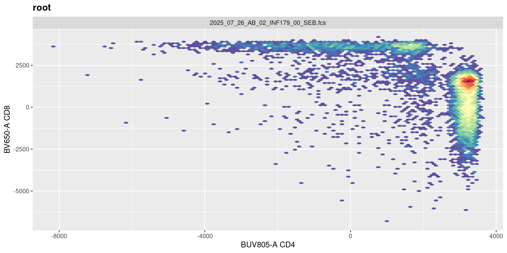
.
We will also need a way to validate whether they are being updated in the background. We can revisit the output of gh_get_transformations() function from earlier, and specify just the first specimen, and the BUV805 fluorophore
function (x, deriv = 0)
{
    deriv <- as.integer(deriv)
    if (deriv < 0 || deriv > 3)
        stop("'deriv' must be between 0 and 3")
    if (deriv > 0) {
        z0 <- double(z$n)
        z[c("y", "b", "c")] <- switch(deriv, list(y = z$b, b = 2 *
            z$c, c = 3 * z$d), list(y = 2 * z$c, b = 6 * z$d,
            c = z0), list(y = 6 * z$d, b = z0, c = z0))
        z[["d"]] <- z0
    }
    res <- stats:::.splinefun(x, z)
    if (deriv > 0 && z$method == 2 && any(ind <- x <= z$x[1L]))
        res[ind] <- ifelse(deriv == 1, z$y[1L], 0)
    res
}
<bytecode: 0x55865e4e3600>
<environment: 0x558650256240>
attr(,"type")
[1] "biexp"
attr(,"parameters")
attr(,"parameters")$channelRange
[1] 4096

attr(,"parameters")$maxValue
[1] 262144

attr(,"parameters")$neg
[1] 0

attr(,"parameters")$pos
[1] 4.5

attr(,"parameters")$widthBasis
[1] -10
width
.
Before we go messing with any of the other setting, let’s tackle width, which tends to be the one that gets missed by the default most often. Normally, in FlowJo most of my plots are set with biexponential transform width of around -1000, so lets go ahead and switch in that value.
SFC_cytoset <- load_cytoset_from_fcs(SFC_files,
 truncate_max_range = FALSE, transformation = FALSE)
SFC_GatingSet <- GatingSet(SFC_cytoset)
Biexponential <- flowjo_biexp_trans(channelRange=4096, maxValue=262144,
     pos=4.5, neg=0, widthBasis=-1000)
MyBiexTransform <- transformerList(FluorophoresOnly, Biexponential)
transform(SFC_GatingSet, MyBiexTransform)
A GatingSet with 6 samples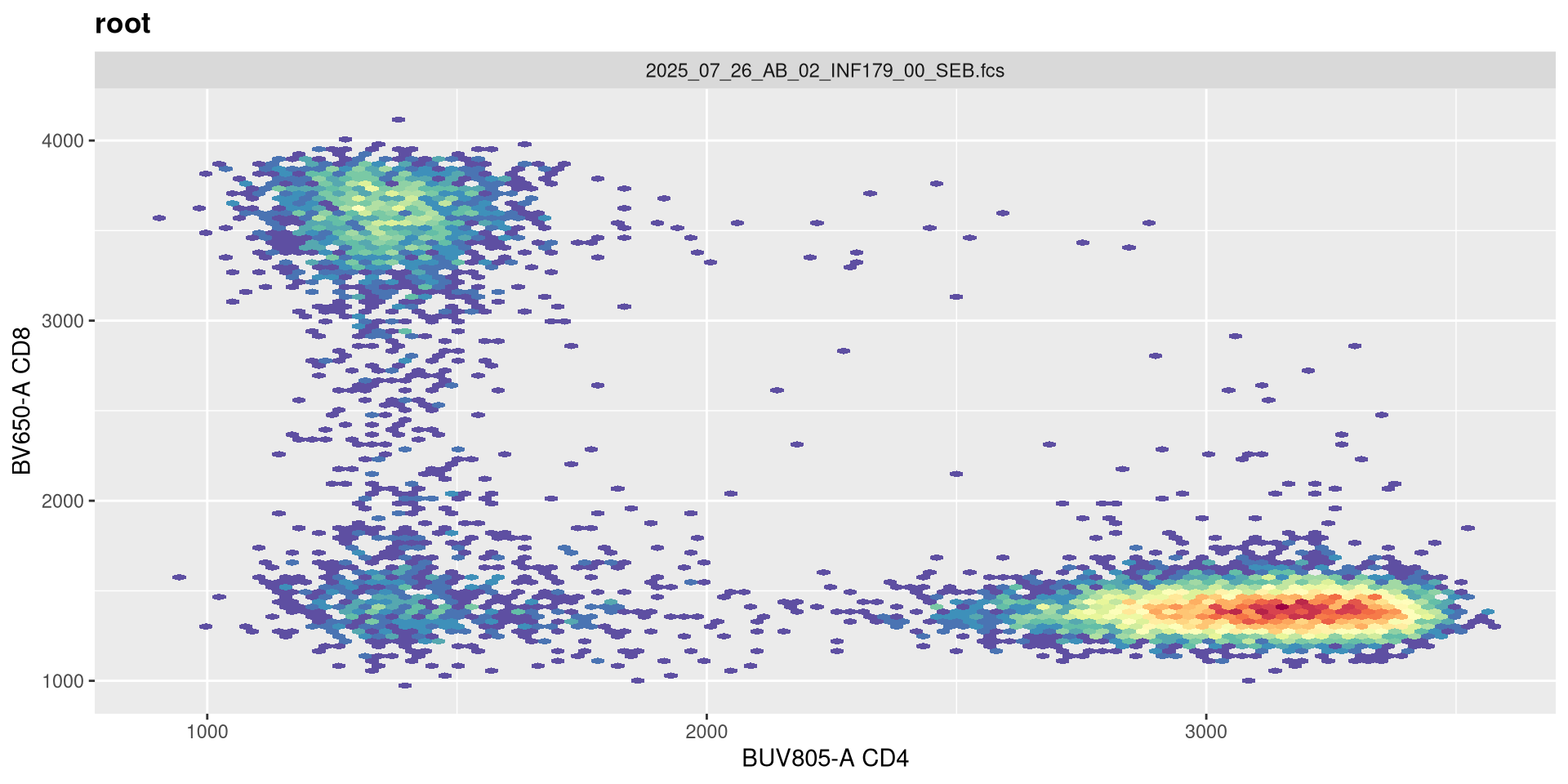
.
Boom! That is more in line with what we were looking for. Let’s still check a couple other values.
SFC_cytoset <- load_cytoset_from_fcs(SFC_files,
 truncate_max_range = FALSE, transformation = FALSE)
SFC_GatingSet <- GatingSet(SFC_cytoset)
Biexponential <- flowjo_biexp_trans(channelRange=4096, maxValue=262144,
     pos=4.5, neg=0, widthBasis=-500)
MyBiexTransform <- transformerList(FluorophoresOnly, Biexponential)
transform(SFC_GatingSet, MyBiexTransform)
A GatingSet with 6 samples
.
A width value of -500 still has the negavite population relative condensed, with the CD4+ cells into a more circular format. Lets try -100 next
SFC_cytoset <- load_cytoset_from_fcs(SFC_files,
 truncate_max_range = FALSE, transformation = FALSE)
SFC_GatingSet <- GatingSet(SFC_cytoset)
Biexponential <- flowjo_biexp_trans(channelRange=4096, maxValue=262144,
     pos=4.5, neg=0, widthBasis=-100)
MyBiexTransform <- transformerList(FluorophoresOnly, Biexponential)
transform(SFC_GatingSet, MyBiexTransform)
A GatingSet with 6 samples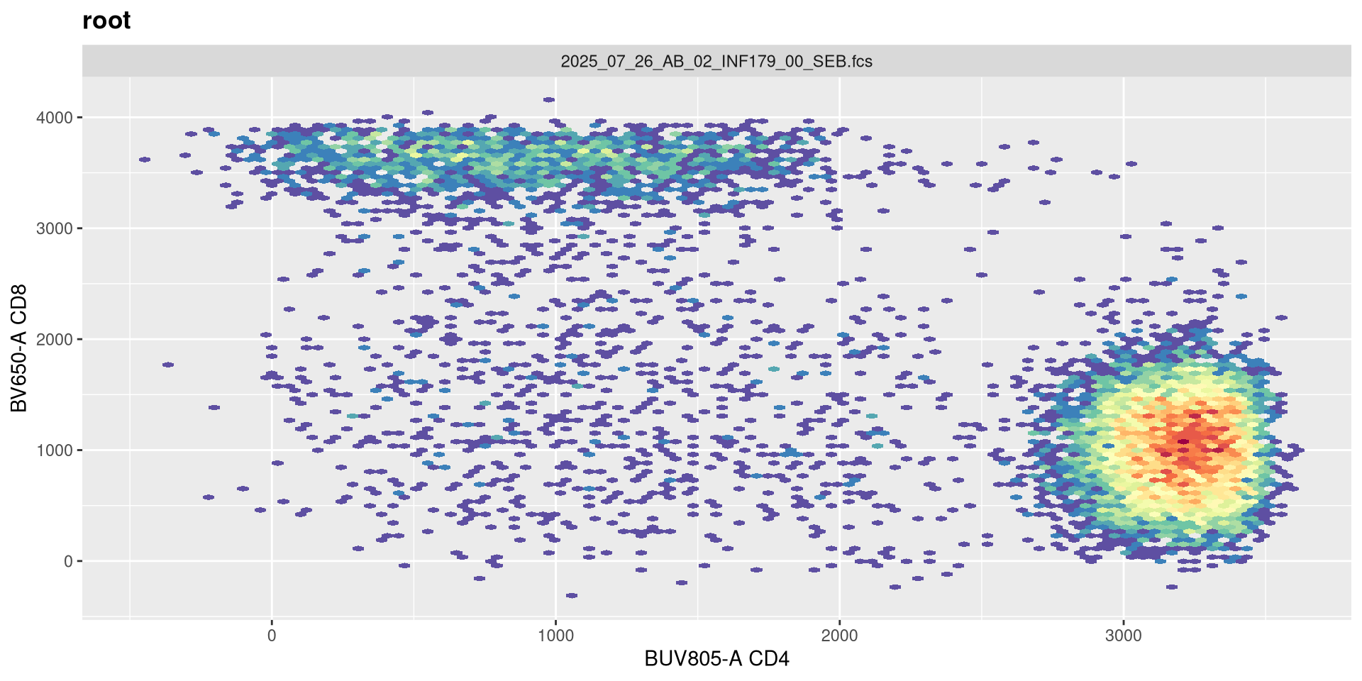
.
And nope, too far. Let’s keep -500 for now.
channelRange
.
Now that width is set closer to what we would expect, lets alter the next couple arguments and see if they have any effect. The argument channelRange is currently set for 4096. Lets double it
SFC_cytoset <- load_cytoset_from_fcs(SFC_files,
 truncate_max_range = FALSE, transformation = FALSE)
SFC_GatingSet <- GatingSet(SFC_cytoset)
Biexponential <- flowjo_biexp_trans(channelRange=8192, maxValue=262144,
     pos=4.5, neg=0, widthBasis=-500)
MyBiexTransform <- transformerList(FluorophoresOnly, Biexponential)
transform(SFC_GatingSet, MyBiexTransform)
A GatingSet with 6 samples
function (x, deriv = 0)
{
    deriv <- as.integer(deriv)
    if (deriv < 0 || deriv > 3)
        stop("'deriv' must be between 0 and 3")
    if (deriv > 0) {
        z0 <- double(z$n)
        z[c("y", "b", "c")] <- switch(deriv, list(y = z$b, b = 2 *
            z$c, c = 3 * z$d), list(y = 2 * z$c, b = 6 * z$d,
            c = z0), list(y = 6 * z$d, b = z0, c = z0))
        z[["d"]] <- z0
    }
    res <- stats:::.splinefun(x, z)
    if (deriv > 0 && z$method == 2 && any(ind <- x <= z$x[1L]))
        res[ind] <- ifelse(deriv == 1, z$y[1L], 0)
    res
}
<bytecode: 0x55865e4e3600>
<environment: 0x5586649fd1e0>
attr(,"type")
[1] "biexp"
attr(,"parameters")
attr(,"parameters")$channelRange
[1] 8192

attr(,"parameters")$maxValue
[1] 262144

attr(,"parameters")$neg
[1] 0

attr(,"parameters")$pos
[1] 4.5

attr(,"parameters")$widthBasis
[1] -500
.
Not much apparent change, so lets go the opposite direction and reduce the original value by half.
SFC_cytoset <- load_cytoset_from_fcs(SFC_files,
 truncate_max_range = FALSE, transformation = FALSE)
SFC_GatingSet <- GatingSet(SFC_cytoset)
Biexponential <- flowjo_biexp_trans(channelRange=2048, maxValue=262144,
     pos=4.5, neg=0, widthBasis=-500)
MyBiexTransform <- transformerList(FluorophoresOnly, Biexponential)
transform(SFC_GatingSet, MyBiexTransform)
A GatingSet with 6 samples
function (x, deriv = 0)
{
    deriv <- as.integer(deriv)
    if (deriv < 0 || deriv > 3)
        stop("'deriv' must be between 0 and 3")
    if (deriv > 0) {
        z0 <- double(z$n)
        z[c("y", "b", "c")] <- switch(deriv, list(y = z$b, b = 2 *
            z$c, c = 3 * z$d), list(y = 2 * z$c, b = 6 * z$d,
            c = z0), list(y = 6 * z$d, b = z0, c = z0))
        z[["d"]] <- z0
    }
    res <- stats:::.splinefun(x, z)
    if (deriv > 0 && z$method == 2 && any(ind <- x <= z$x[1L]))
        res[ind] <- ifelse(deriv == 1, z$y[1L], 0)
    res
}
<bytecode: 0x55865e4e3600>
<environment: 0x558651cc5080>
attr(,"type")
[1] "biexp"
attr(,"parameters")
attr(,"parameters")$channelRange
[1] 2048

attr(,"parameters")$maxValue
[1] 262144

attr(,"parameters")$neg
[1] 0

attr(,"parameters")$pos
[1] 4.5

attr(,"parameters")$widthBasis
[1] -500
.
Few minor changes, but not much otherwise. So lets proceed on to the next argument!
maxValue
.
Same procedure, the current maxValue is 262144, lets double it and see what happens!
SFC_cytoset <- load_cytoset_from_fcs(SFC_files,
 truncate_max_range = FALSE, transformation = FALSE)
SFC_GatingSet <- GatingSet(SFC_cytoset)
Biexponential <- flowjo_biexp_trans(channelRange=4096, maxValue=524288,
     pos=4.5, neg=0, widthBasis=-500)
MyBiexTransform <- transformerList(FluorophoresOnly, Biexponential)
transform(SFC_GatingSet, MyBiexTransform)
A GatingSet with 6 samples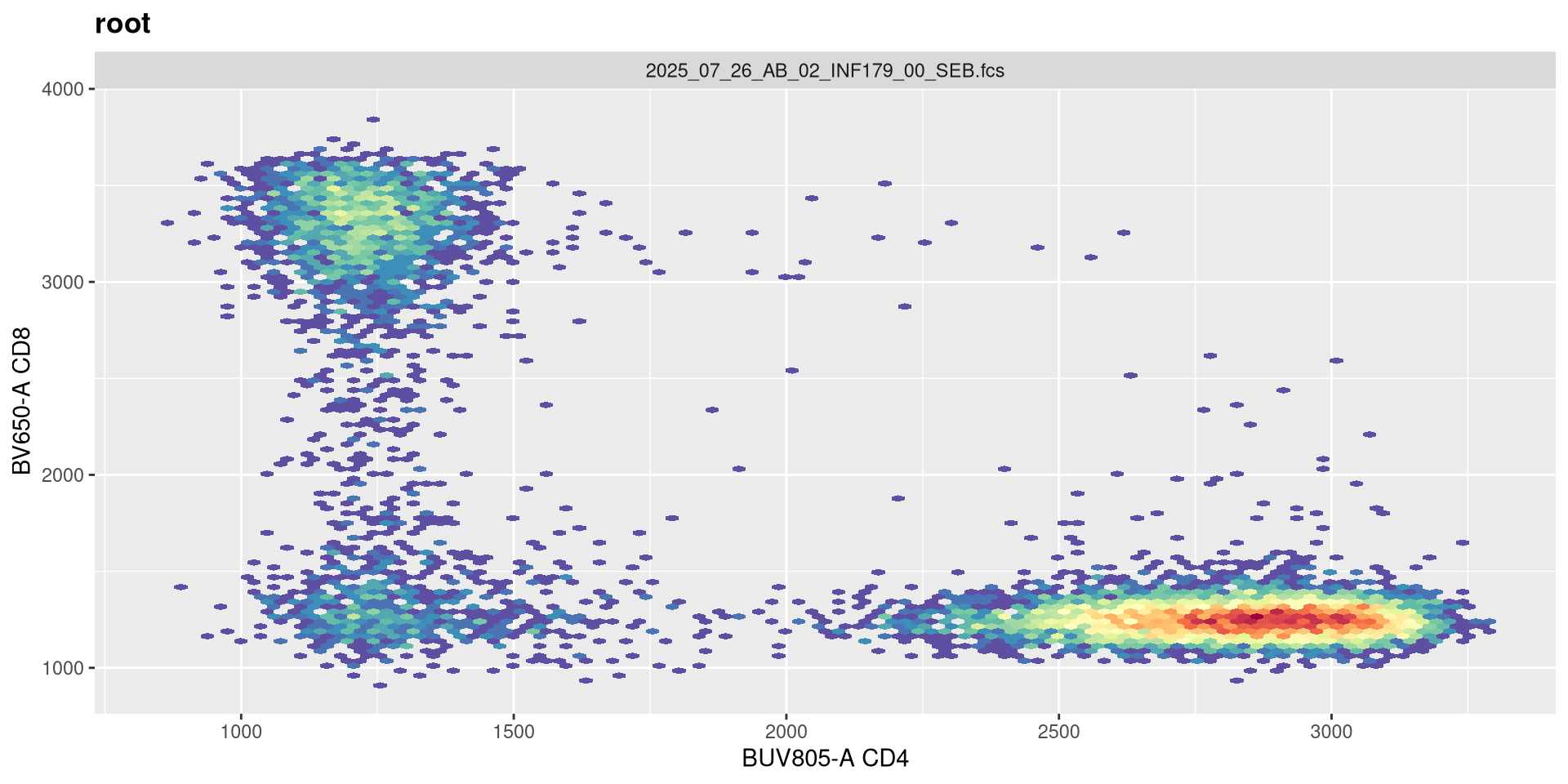
.
You will notice, that when we doubled the maxValue, we are phenocopying the result we got when we had width set to -1000, with the CD4 population. This is worth noting. Lets now try instead to reduce it!
SFC_cytoset <- load_cytoset_from_fcs(SFC_files,
 truncate_max_range = FALSE, transformation = FALSE)
SFC_GatingSet <- GatingSet(SFC_cytoset)
Biexponential <- flowjo_biexp_trans(channelRange=4096, maxValue=131072,
     pos=4.5, neg=0, widthBasis=-500)
MyBiexTransform <- transformerList(FluorophoresOnly, Biexponential)
transform(SFC_GatingSet, MyBiexTransform)
A GatingSet with 6 samples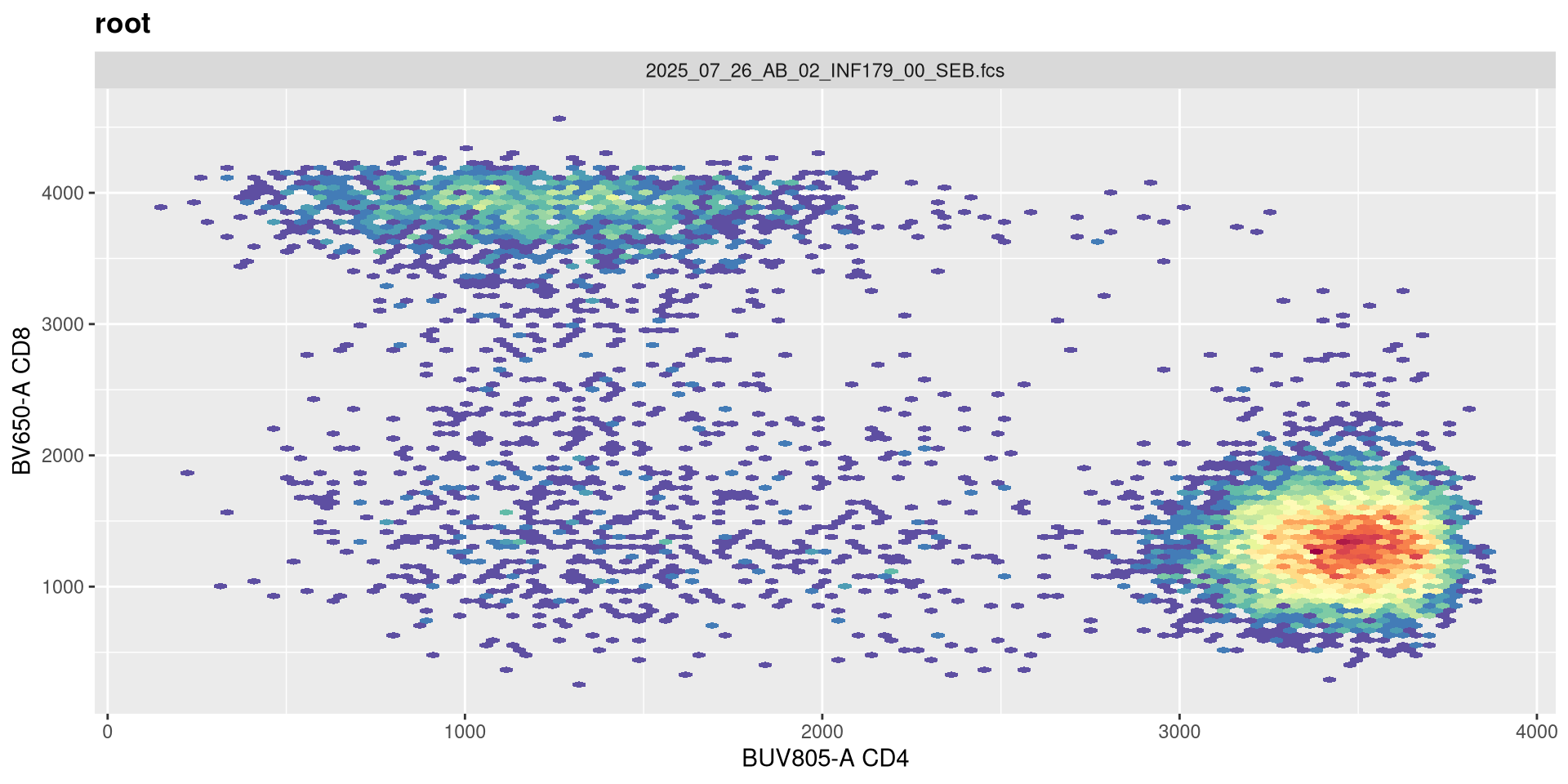
.
And likewise, we are going the opposite to our intended effect. As maxValue can in part be determined by our instrument settings (as well as individual fluorophores), this is an argument we should keep an eye on. Let’s leave it at its current default for now.
pos
.
The next argument pos corresponds to the number of positive decades. It is currently set at 4.5
SFC_cytoset <- load_cytoset_from_fcs(SFC_files,
 truncate_max_range = FALSE, transformation = FALSE)
SFC_GatingSet <- GatingSet(SFC_cytoset)
Biexponential <- flowjo_biexp_trans(channelRange=4096, maxValue=262144,
     pos=4.5, neg=0, widthBasis=-500)
MyBiexTransform <- transformerList(FluorophoresOnly, Biexponential)
transform(SFC_GatingSet, MyBiexTransform)
A GatingSet with 6 samples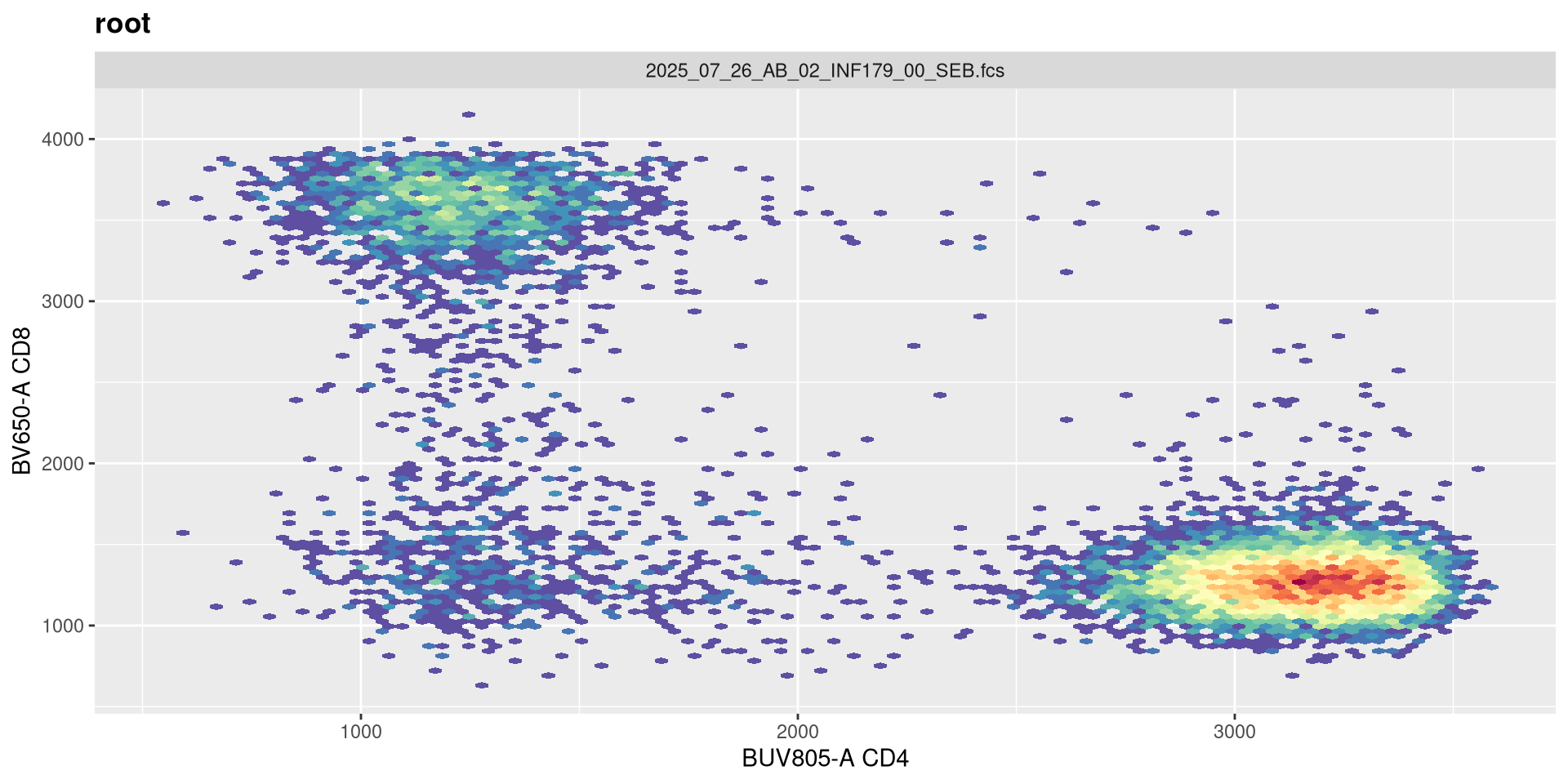
.
Although this can be increased on some instrument settings. Let’s walk it up to 5!
SFC_cytoset <- load_cytoset_from_fcs(SFC_files,
 truncate_max_range = FALSE, transformation = FALSE)
SFC_GatingSet <- GatingSet(SFC_cytoset)
Biexponential <- flowjo_biexp_trans(channelRange=4096, maxValue=262144,
     pos=5, neg=0, widthBasis=-500)
MyBiexTransform <- transformerList(FluorophoresOnly, Biexponential)
transform(SFC_GatingSet, MyBiexTransform)
A GatingSet with 6 samples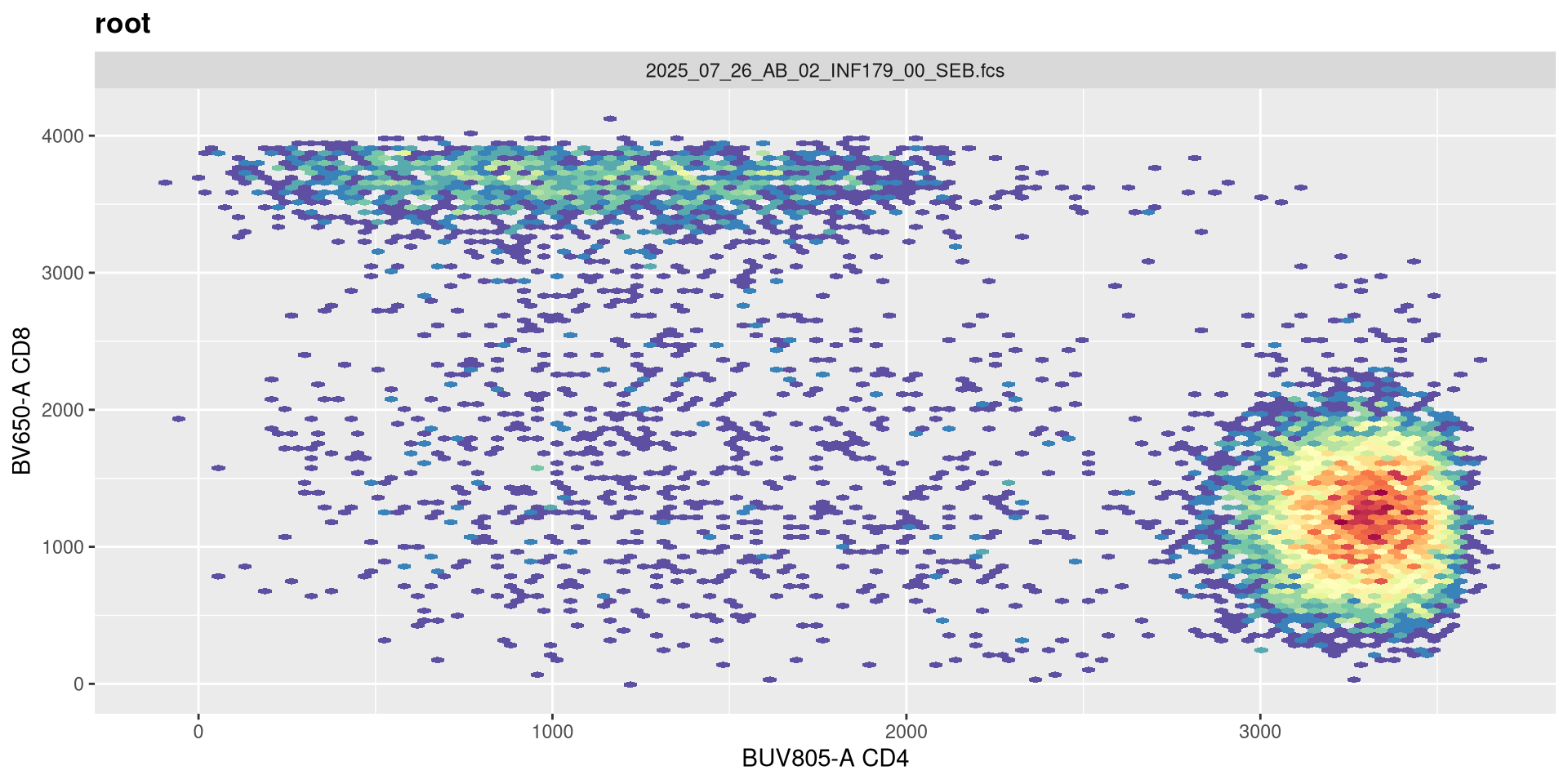
.
And on first glance no. If we had our settings for 5 positive decades, we would need to adjust both the maxValue and widthBasis to return to a closer to expected shape.
SFC_cytoset <- load_cytoset_from_fcs(SFC_files,
 truncate_max_range = FALSE, transformation = FALSE)
SFC_GatingSet <- GatingSet(SFC_cytoset)
Biexponential <- flowjo_biexp_trans(channelRange=4096, maxValue=524288,
     pos=5, neg=0, widthBasis=-1000)
MyBiexTransform <- transformerList(FluorophoresOnly, Biexponential)
transform(SFC_GatingSet, MyBiexTransform)
A GatingSet with 6 samples
neg
.
We have a similar story for adding negative decades.
SFC_cytoset <- load_cytoset_from_fcs(SFC_files,
 truncate_max_range = FALSE, transformation = FALSE)
SFC_GatingSet <- GatingSet(SFC_cytoset)
Biexponential <- flowjo_biexp_trans(channelRange=4096, maxValue=262144,
     pos=4.5, neg=0, widthBasis=-500)
MyBiexTransform <- transformerList(FluorophoresOnly, Biexponential)
transform(SFC_GatingSet, MyBiexTransform)
A GatingSet with 6 samples
.
Adding an extra negative decade doesn’t seem to noticiblt affect these two fluorophores.
SFC_cytoset <- load_cytoset_from_fcs(SFC_files,
 truncate_max_range = FALSE, transformation = FALSE)
SFC_GatingSet <- GatingSet(SFC_cytoset)
Biexponential <- flowjo_biexp_trans(channelRange=4096, maxValue=262144,
     pos=4.5, neg=1, widthBasis=-500)
MyBiexTransform <- transformerList(FluorophoresOnly, Biexponential)
transform(SFC_GatingSet, MyBiexTransform)
A GatingSet with 6 samples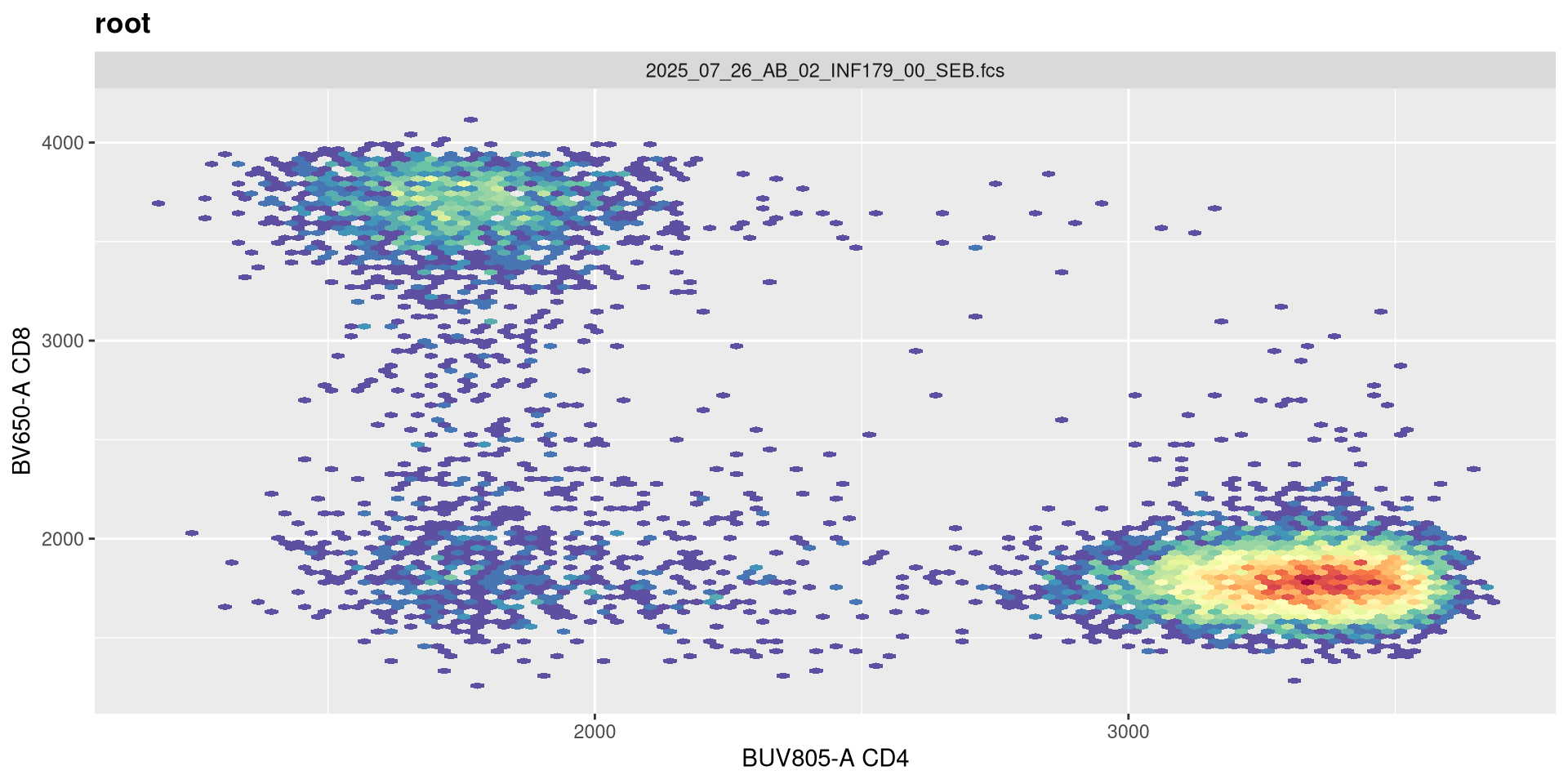
.
It is only when we increase to 2 (i.e. -2 decades) that we start to see a spreading effect.
SFC_cytoset <- load_cytoset_from_fcs(SFC_files,
 truncate_max_range = FALSE, transformation = FALSE)
SFC_GatingSet <- GatingSet(SFC_cytoset)
Biexponential <- flowjo_biexp_trans(channelRange=4096, maxValue=262144,
     pos=4.5, neg=2, widthBasis=-500)
MyBiexTransform <- transformerList(FluorophoresOnly, Biexponential)
transform(SFC_GatingSet, MyBiexTransform)
A GatingSet with 6 samples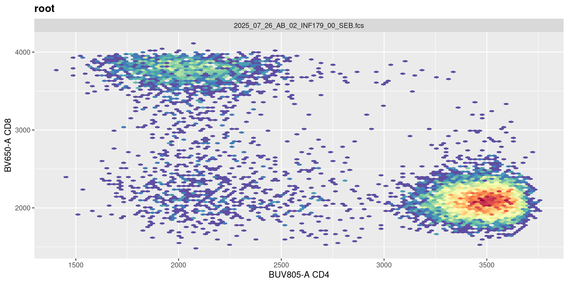
Recap
.
We have looked at how the various arguments can affect the overall visualization, and seen how some of these are interconnected. It might be worthwhile to verify what your own instrument settings are at first (especially in context of maxValue and positive decades), and then use these when starting in R for the first time.
MC
.
Having now had some experience applying transformations to SFC data, let’s turn and look at how to apply arsinh to our mass cytometry (CyTOF) dataset. Lets once again make sure we have the correct .fcs files
.
And modify the steps from Week 05 to load them into a GatingSet object.
.
Let’s examine the names for the metal tags
 [1] "Ce140Di"      "Ce142Di"      "Dy161Di"      "Dy162Di"      "Dy163Di"
 [6] "Dy164Di"      "Er166Di"      "Er167Di"      "Er168Di"      "Er170Di"
[11] "Eu151Di"      "Eu153Di"      "Event_length" "Gd155Di"      "Gd156Di"
[16] "Gd158Di"      "Gd160Di"      "Ho165Di"      "Ir191Di"      "Ir193Di"
[21] "Lu175Di"      "Lu176Di"      "Nd142Di"      "Nd143Di"      "Nd144Di"
[26] "Nd145Di"      "Nd146Di"      "Nd148Di"      "Nd150Di"      "Pd102Di"
[31] "Pd104Di"      "Pd105Di"      "Pd106Di"      "Pd108Di"      "Pd110Di"
[36] "Pr141Di"      "Pt195Di"      "Sm147Di"      "Sm149Di"      "Sm152Di"
[41] "Sm154Di"      "Tb159Di"      "Tm169Di"      "Y89Di"        "Yb171Di"
[46] "Yb172Di"      "Yb173Di"      "Yb174Di"      "Yb176Di"      "Time"
.
And the corresponding markers associated with each
               Ce140Di                Ce142Di                Dy161Di
               "Beads"                "Beads"   "H2BK120Ub-macroH2A"
               Dy162Di                Dy163Di                Dy164Di
   "CrotonylK-H3K4me3"        "H3R2cit-H2A.Z"     "H3K14ac-H3K36me1"
               Er166Di                Er167Di                Er168Di
                "CD33"                 "CD16"     "H4K16ac-H4K20me1"
               Er170Di                Eu151Di                Eu153Di
                 "CD3"     "H3K23ac-H3K27me1"    "H2BS14ph-H3K36me2"
               Gd155Di                Gd156Di                Gd158Di
               "CD11c"     "H3K18ac-H4K20me2"         "H3K56ac-H3.3"
               Gd160Di                Ho165Di                Ir191Di
      "PADI4-H4K20me3"     "H33Xcit-H3K27me3"                  "DNA"
               Ir193Di                Lu175Di                Lu176Di
                 "DNA"                 "CD19"                "beads"
               Nd142Di                Nd143Di                Nd144Di
      "gammaH2AX-Rme1"      "H2BK5ac-Rme2sym"      "H3S10ph-H3K4me2"
               Nd145Di                Nd146Di                Nd148Di
                 "CD4"                  "CD8"                 "CD34"
               Nd150Di                Pd102Di                Pd104Di
  "H3.3S31ph-H3K36me3"              "Barcode"              "Barcode"
               Pd105Di                Pd106Di                Pd108Di
             "Barcode"              "Barcode"              "Barcode"
               Pd110Di                Pr141Di                Pt195Di
             "Barcode"                   "H3"             "livedead"
               Sm147Di                Sm149Di                Sm152Di
      "H4K5ac-H3K9me2" "CleavedH3T22-H3K9me1"       "H3K9ac-Rme2asy"
               Sm154Di                Tb159Di                Tm169Di
  "H2AK119Ub-H3K27me2"                 "CD14"                "CD123"
                 Y89Di                Yb171Di                Yb172Di
                "CD45"                 "CD38"                 "CD56"
               Yb173Di                Yb174Di                Yb176Di
                  "H4"        "H3K27ac-CENPA"                "HLADR"
.
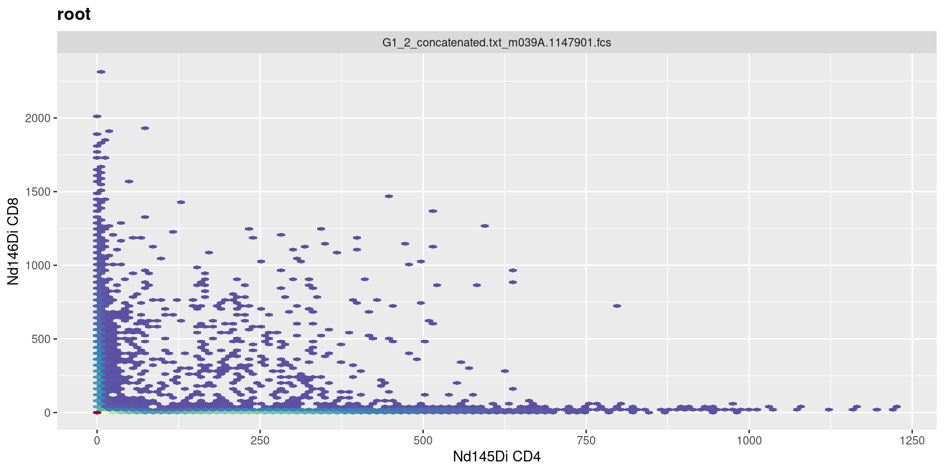
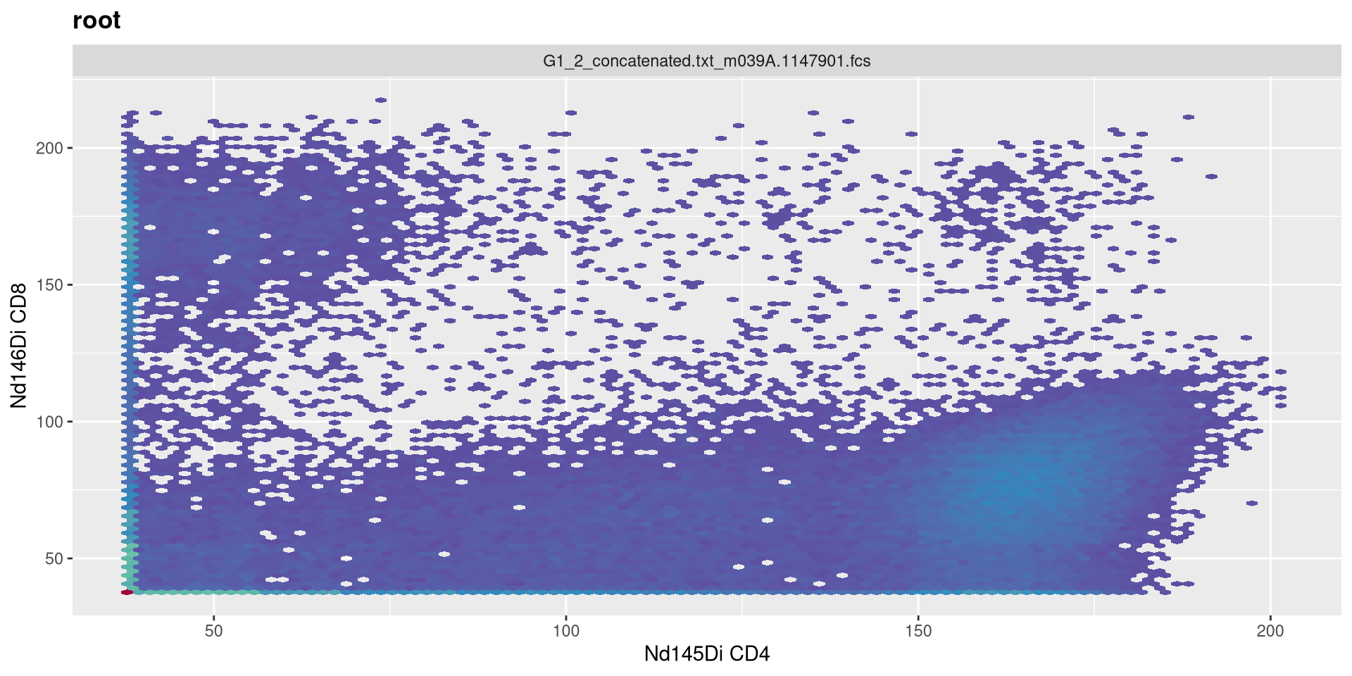
And lets go ahead and visualize the CD4 x CD8 plot for the first specimen.
.
We can then select the particular markers we are interested, that we want to end up transforming. For this example, lets say we wanted to remove the multiple Barcode and Beads entries
               Dy161Di                Dy162Di                Dy163Di
  "H2BK120Ub-macroH2A"    "CrotonylK-H3K4me3"        "H3R2cit-H2A.Z"
               Dy164Di                Er166Di                Er167Di
    "H3K14ac-H3K36me1"                 "CD33"                 "CD16"
               Er168Di                Er170Di                Eu151Di
    "H4K16ac-H4K20me1"                  "CD3"     "H3K23ac-H3K27me1"
               Eu153Di                Gd155Di                Gd156Di
   "H2BS14ph-H3K36me2"                "CD11c"     "H3K18ac-H4K20me2"
               Gd158Di                Gd160Di                Ho165Di
        "H3K56ac-H3.3"       "PADI4-H4K20me3"     "H33Xcit-H3K27me3"
               Ir191Di                Ir193Di                Lu175Di
                 "DNA"                  "DNA"                 "CD19"
               Lu176Di                Nd142Di                Nd143Di
               "beads"       "gammaH2AX-Rme1"      "H2BK5ac-Rme2sym"
               Nd144Di                Nd145Di                Nd146Di
     "H3S10ph-H3K4me2"                  "CD4"                  "CD8"
               Nd148Di                Nd150Di                Pr141Di
                "CD34"   "H3.3S31ph-H3K36me3"                   "H3"
               Pt195Di                Sm147Di                Sm149Di
            "livedead"       "H4K5ac-H3K9me2" "CleavedH3T22-H3K9me1"
               Sm152Di                Sm154Di                Tb159Di
      "H3K9ac-Rme2asy"   "H2AK119Ub-H3K27me2"                 "CD14"
               Tm169Di                  Y89Di                Yb171Di
               "CD123"                 "CD45"                 "CD38"
               Yb172Di                Yb173Di                Yb174Di
                "CD56"                   "H4"        "H3K27ac-CENPA"
               Yb176Di
               "HLADR"
.
Of which, we want the names for this named list. So….
 [1] "Dy161Di" "Dy162Di" "Dy163Di" "Dy164Di" "Er166Di" "Er167Di" "Er168Di"
 [8] "Er170Di" "Eu151Di" "Eu153Di" "Gd155Di" "Gd156Di" "Gd158Di" "Gd160Di"
[15] "Ho165Di" "Ir191Di" "Ir193Di" "Lu175Di" "Lu176Di" "Nd142Di" "Nd143Di"
[22] "Nd144Di" "Nd145Di" "Nd146Di" "Nd148Di" "Nd150Di" "Pr141Di" "Pt195Di"
[29] "Sm147Di" "Sm149Di" "Sm152Di" "Sm154Di" "Tb159Di" "Tm169Di" "Y89Di"
[36] "Yb171Di" "Yb172Di" "Yb173Di" "Yb174Di" "Yb176Di"
.
With these, we can then combine them with our transformer of interest to create the transformerList() that we can then apply to the samples.
List of 3
 $ Dy161Di:List of 9
  ..$ name        : chr "flowJo_fasinh"
  ..$ transform   :function (x)
  ..$ inverse     :function (x)
  ..$ d_transform : NULL
  ..$ d_inverse   : NULL
  ..$ breaks      :function (x)
  ..$ minor_breaks:function (b, limits, n)
  ..$ format      :function (x)
  ..$ domain      : num [1:2] -Inf Inf
  ..- attr(*, "class")= chr "transform"
 $ Dy162Di:List of 9
  ..$ name        : chr "flowJo_fasinh"
  ..$ transform   :function (x)
  ..$ inverse     :function (x)
  ..$ d_transform : NULL
  ..$ d_inverse   : NULL
  ..$ breaks      :function (x)
  ..$ minor_breaks:function (b, limits, n)
  ..$ format      :function (x)
  ..$ domain      : num [1:2] -Inf Inf
  ..- attr(*, "class")= chr "transform"
 $ Dy163Di:List of 9
  ..$ name        : chr "flowJo_fasinh"
  ..$ transform   :function (x)
  ..$ inverse     :function (x)
  ..$ d_transform : NULL
  ..$ d_inverse   : NULL
  ..$ breaks      :function (x)
  ..$ minor_breaks:function (b, limits, n)
  ..$ format      :function (x)
  ..$ domain      : num [1:2] -Inf Inf
..- attr(*, "class")= chr "transform".
With this done, let’s try replotting the previous CD4 by CD8 plot
Asinh Arguments
.
Similar to the case with SFC, we may need to revise some of the values provided to the individual arguments. Lets similarly investigate what we can do
.
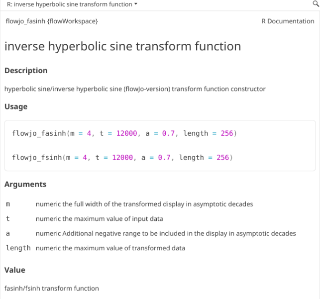
Which turns out to be another wrapper. Lets try the similarly named function
.
As we may remember, our current setting are the following
MC_cytoset <- load_cytoset_from_fcs(MC_files,
 truncate_max_range = FALSE, transformation = FALSE)
MC_GatingSet <- GatingSet(MC_cytoset)
Asinh <- flowjo_fasinh_trans(m = 4, t = 12000, a = 0.7, length = 256)
MyAsinhTransform <- transformerList(InterestingMetalsOnly, Asinh)
transform(MC_GatingSet, MyAsinhTransform)
A GatingSet with 3 samples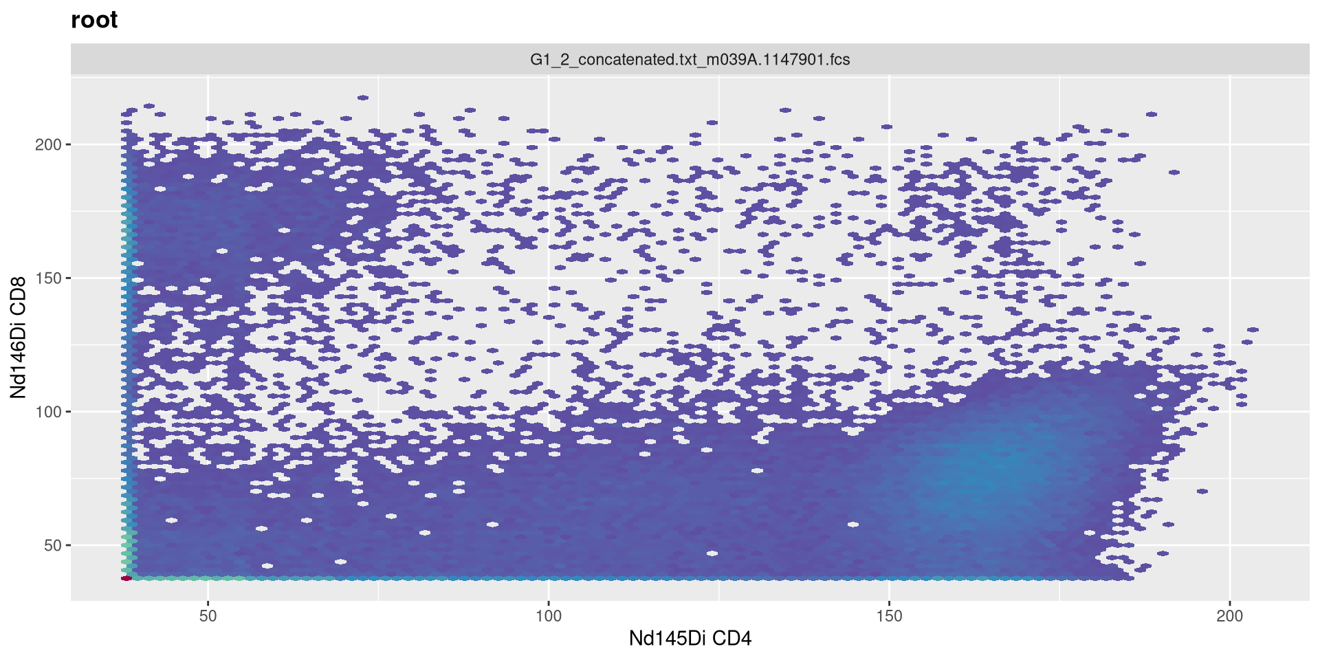
m
.
Being completionist, lets change the MC arguments as well. M is width in asymptotic decades, currently set to 4.
MC_cytoset <- load_cytoset_from_fcs(MC_files,
 truncate_max_range = FALSE, transformation = FALSE)
MC_GatingSet <- GatingSet(MC_cytoset)
Asinh <- flowjo_fasinh_trans(m = 4, t = 12000, a = 0.7, length = 256)
MyAsinhTransform <- transformerList(InterestingMetalsOnly, Asinh)
transform(MC_GatingSet, MyAsinhTransform)
A GatingSet with 3 samples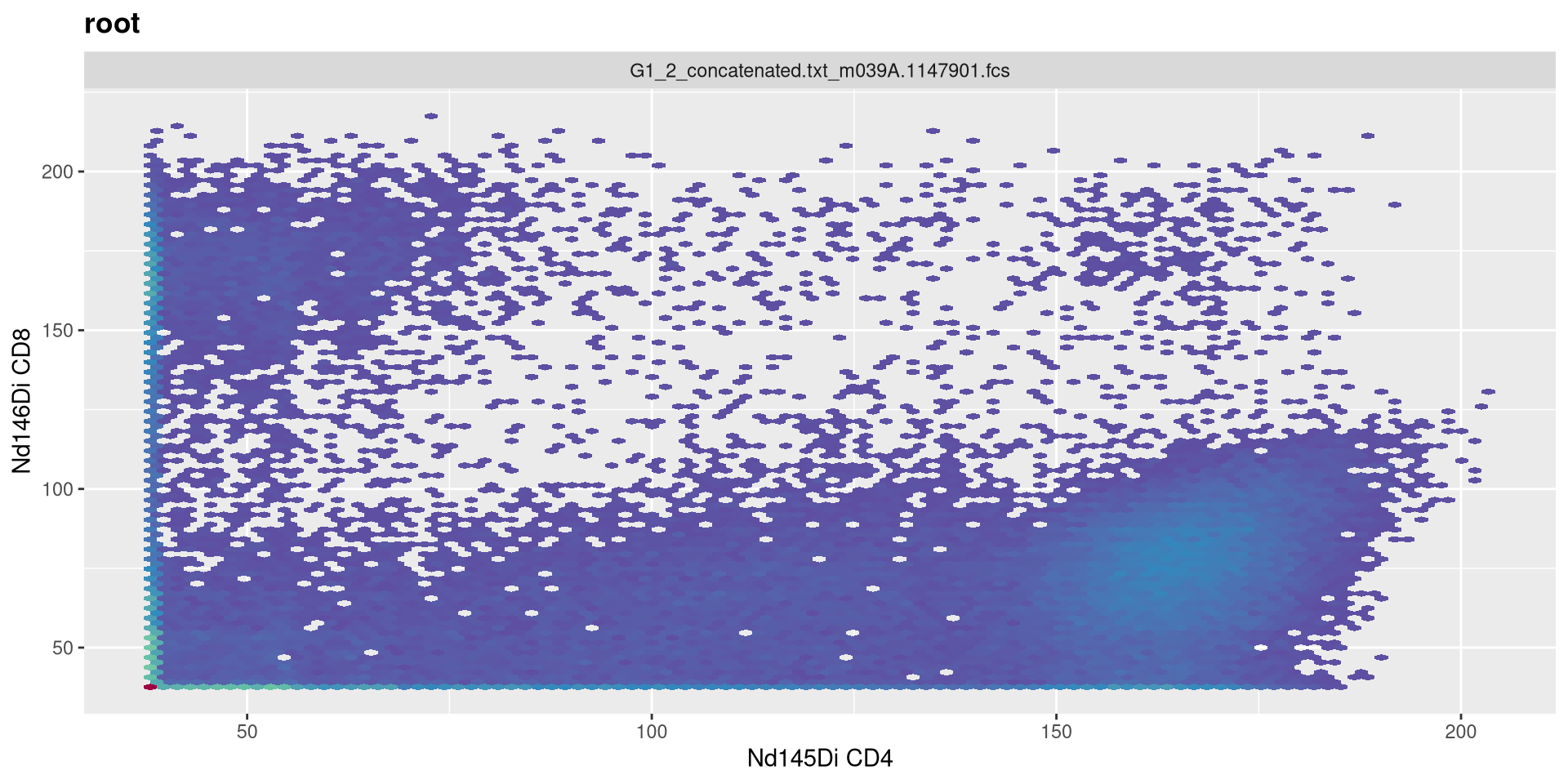
.
Lets set it to 5!
MC_cytoset <- load_cytoset_from_fcs(MC_files,
 truncate_max_range = FALSE, transformation = FALSE)
MC_GatingSet <- GatingSet(MC_cytoset)
Asinh <- flowjo_fasinh_trans(m = 5, t = 12000, a = 0.7, length = 256)
MyAsinhTransform <- transformerList(InterestingMetalsOnly, Asinh)
transform(MC_GatingSet, MyAsinhTransform)
A GatingSet with 3 samples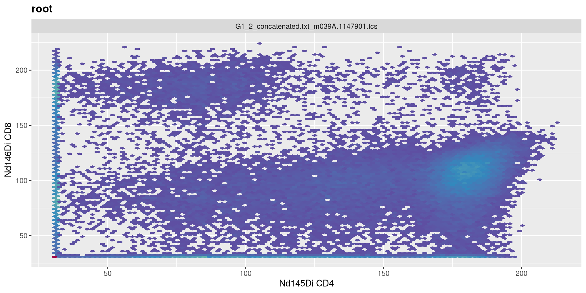
.
Vs. when we set it to 3
MC_cytoset <- load_cytoset_from_fcs(MC_files,
 truncate_max_range = FALSE, transformation = FALSE)
MC_GatingSet <- GatingSet(MC_cytoset)
Asinh <- flowjo_fasinh_trans(m = 3, t = 12000, a = 0.7, length = 256)
MyAsinhTransform <- transformerList(InterestingMetalsOnly, Asinh)
transform(MC_GatingSet, MyAsinhTransform)
A GatingSet with 3 samples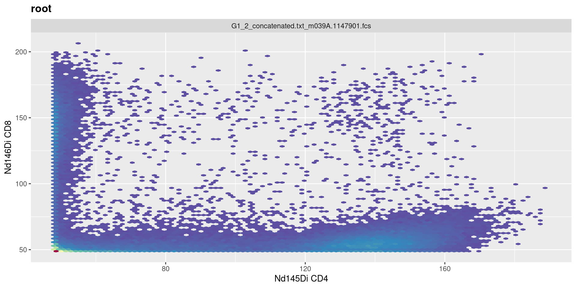
t
.
Increase t to 24000
MC_cytoset <- load_cytoset_from_fcs(MC_files,
 truncate_max_range = FALSE, transformation = FALSE)
MC_GatingSet <- GatingSet(MC_cytoset)
Asinh <- flowjo_fasinh_trans(m = 4, t = 24000, a = 0.7, length = 256)
MyAsinhTransform <- transformerList(InterestingMetalsOnly, Asinh)
transform(MC_GatingSet, MyAsinhTransform)
A GatingSet with 3 samples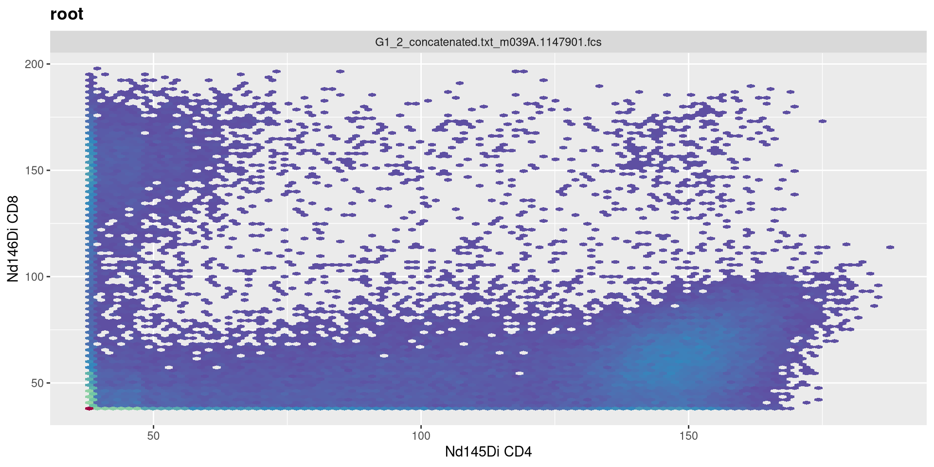
.
Decrease t to 6000
MC_cytoset <- load_cytoset_from_fcs(MC_files,
 truncate_max_range = FALSE, transformation = FALSE)
MC_GatingSet <- GatingSet(MC_cytoset)
Asinh <- flowjo_fasinh_trans(m = 4, t = 6000, a = 0.7, length = 256)
MyAsinhTransform <- transformerList(InterestingMetalsOnly, Asinh)
transform(MC_GatingSet, MyAsinhTransform)
A GatingSet with 3 samples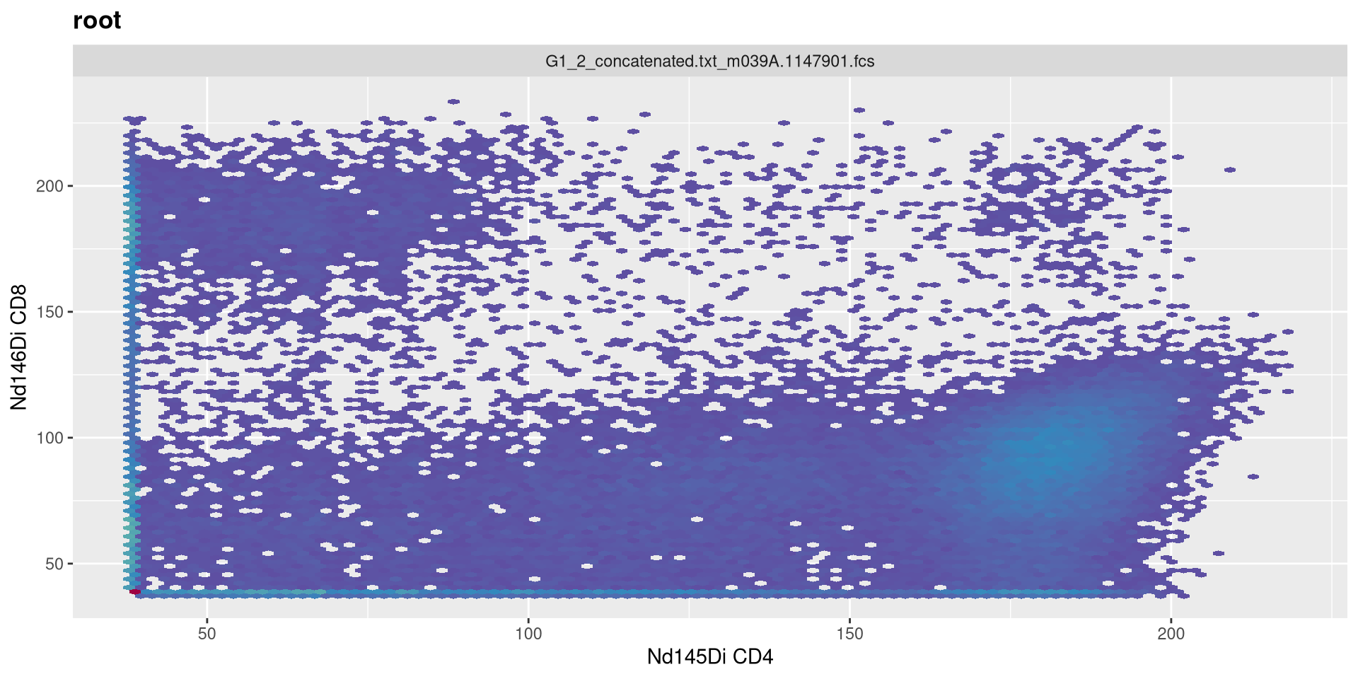
a
.
Increase negative decade to 1
MC_cytoset <- load_cytoset_from_fcs(MC_files,
 truncate_max_range = FALSE, transformation = FALSE)
MC_GatingSet <- GatingSet(MC_cytoset)
Asinh <- flowjo_fasinh_trans(m = 4, t = 12000, a = 1, length = 256)
MyAsinhTransform <- transformerList(InterestingMetalsOnly, Asinh)
transform(MC_GatingSet, MyAsinhTransform)
A GatingSet with 3 samples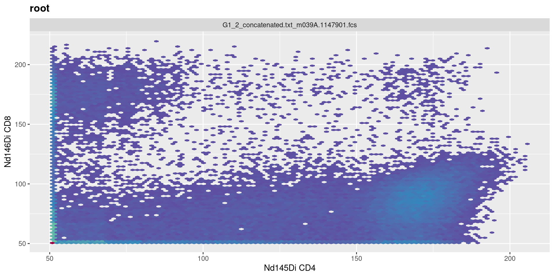
.
Vs. set to 0
MC_cytoset <- load_cytoset_from_fcs(MC_files,
 truncate_max_range = FALSE, transformation = FALSE)
MC_GatingSet <- GatingSet(MC_cytoset)
Asinh <- flowjo_fasinh_trans(m = 4, t = 12000, a = 0, length = 256)
MyAsinhTransform <- transformerList(InterestingMetalsOnly, Asinh)
transform(MC_GatingSet, MyAsinhTransform)
A GatingSet with 3 samples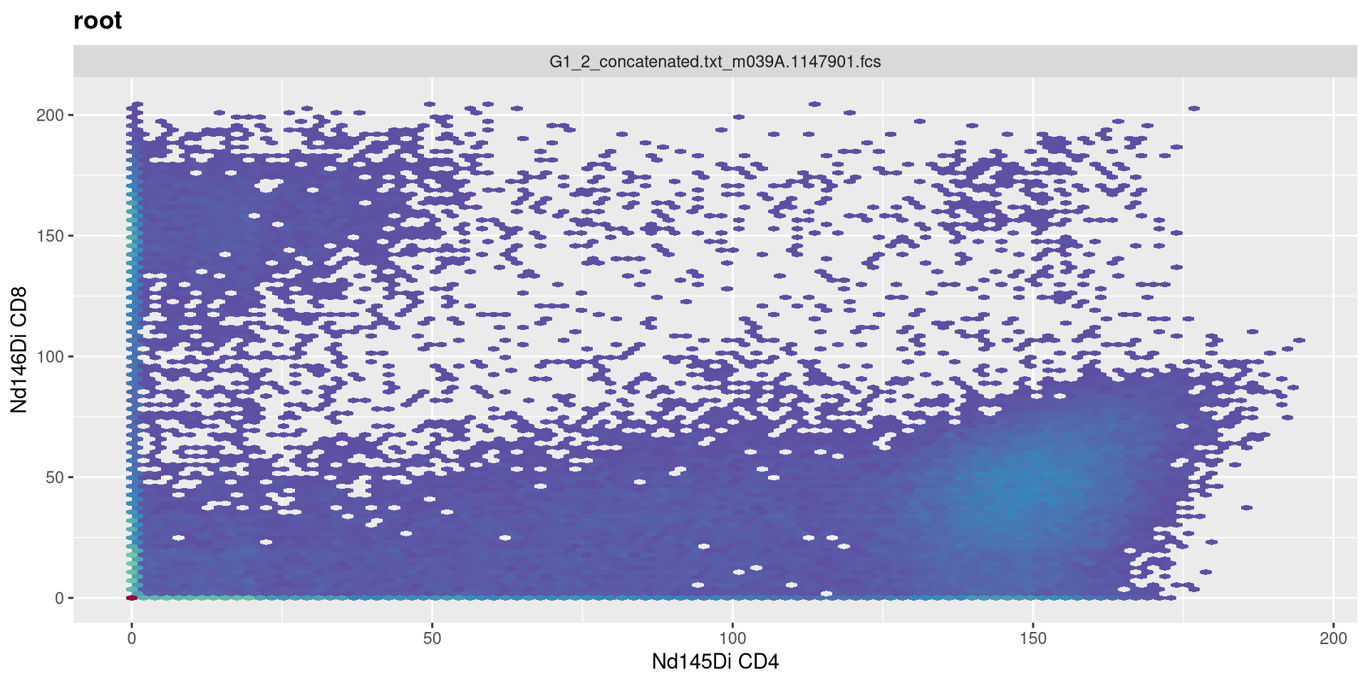
length
.
Doubling numeric max value of transformed data to 512
MC_cytoset <- load_cytoset_from_fcs(MC_files,
 truncate_max_range = FALSE, transformation = FALSE)
MC_GatingSet <- GatingSet(MC_cytoset)
Asinh <- flowjo_fasinh_trans(m = 4, t = 12000, a = 1, length = 512)
MyAsinhTransform <- transformerList(InterestingMetalsOnly, Asinh)
transform(MC_GatingSet, MyAsinhTransform)
A GatingSet with 3 samples
.
Vs. reducing it to 128
MC_cytoset <- load_cytoset_from_fcs(MC_files,
 truncate_max_range = FALSE, transformation = FALSE)
MC_GatingSet <- GatingSet(MC_cytoset)
Asinh <- flowjo_fasinh_trans(m = 4, t = 12000, a = 1, length = 128)
MyAsinhTransform <- transformerList(InterestingMetalsOnly, Asinh)
transform(MC_GatingSet, MyAsinhTransform)
A GatingSet with 3 samples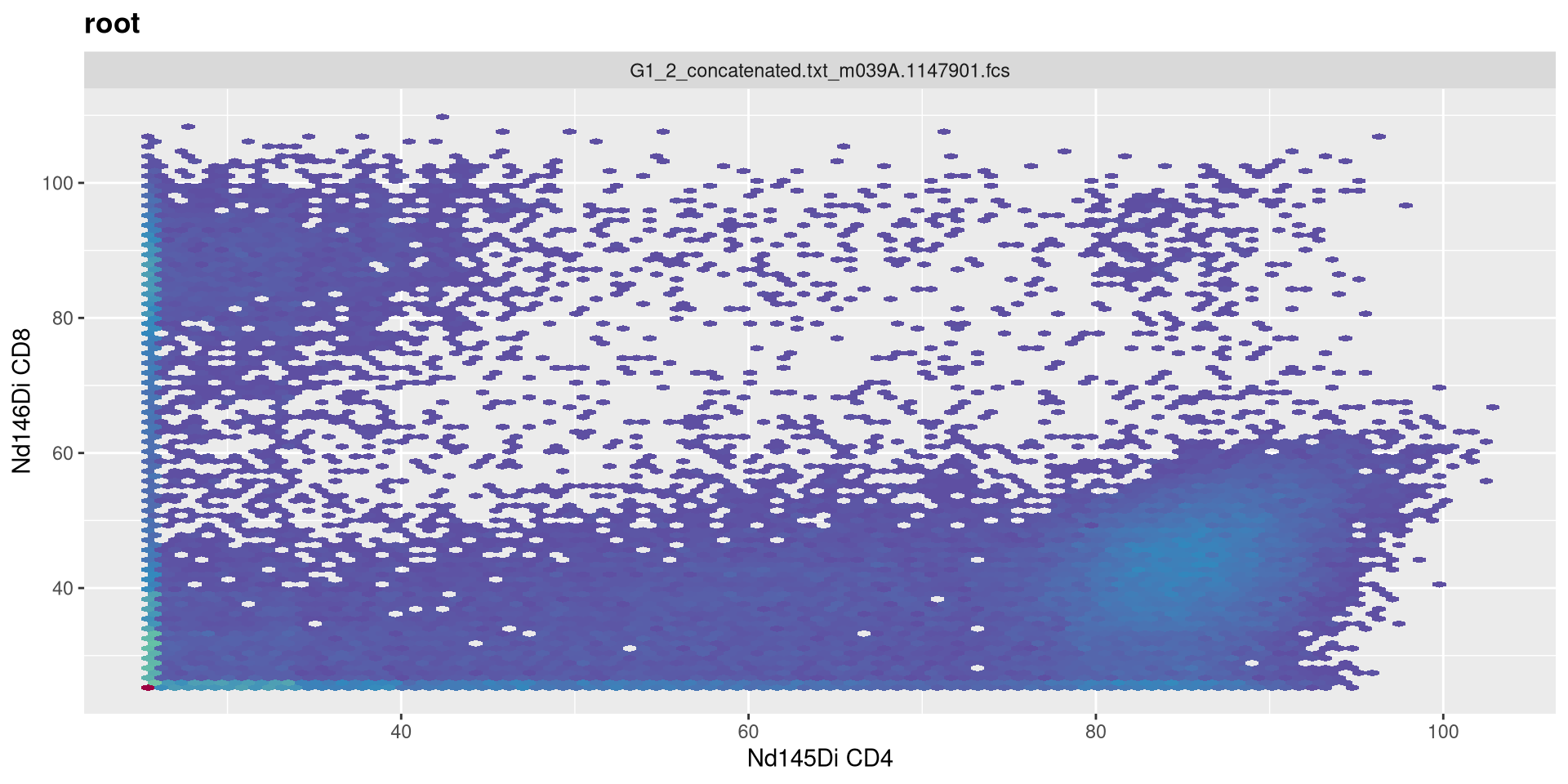
Extracting Data
.
One area where we will separately need to remember whether a transformation is applied or not is later on in the course, when we are trying to extract out the underlying exprs data for use in downstream analysis. If we wanted to do this for our current GatingSet, we first need to fetch the pointer contents to return a CytoSet object.
A cytoset with 1 samples.

  column names:
    Time, SSC-W, SSC-H, SSC-A, FSC-W, FSC-H, FSC-A, SSC-B-W, SSC-B-H, SSC-B-A, BUV395-A, BUV563-A, BUV615-A, BUV661-A, BUV737-A, BUV805-A, Pacific Blue-A, BV480-A, BV570-A, BV605-A, BV650-A, BV711-A, BV750-A, BV786-A, Alexa Fluor 488-A, Spark Blue 550-A, Spark Blue 574-A, RB613-A, RB705-A, RB780-A, PE-A, PE-Dazzle594-A, PE-Cy5-A, PE-Fire 700-A, PE-Fire 744-A, PE-Vio770-A, APC-A, Alexa Fluor 647-A, APC-R700-A, Zombie NIR-A, APC-Fire 750-A, APC-Fire 810-A, AF-A

cytoset has been subsetted and can be realized through 'realize_view()'.
.
We can then extract our the underlying MFI data using the exprs() function.
         Time    SSC-W  SSC-H    SSC-A    FSC-W   FSC-H   FSC-A  SSC-B-W
[1,] 396.1327 741155.4 495200 611700.2 735140.7 1398530 1713527 715626.7
[2,] 539.4743 730091.3 504832 614289.1 714323.2 1607285 1913535 728604.2
[3,] 590.1619 842852.1 267735 376101.7 715528.4  824483  983235 781794.9
     SSC-B-H  SSC-B-A BUV395-A BUV563-A BUV615-A BUV661-A BUV737-A BUV805-A
[1,]  416383 496624.7 3150.359 2315.777 2182.396 2132.781 2889.922 3597.062
[2,]  385314 467902.4 2064.067 3614.399 2124.969 1805.567 2639.037 1866.229
[3,]  309681 403511.7 3336.325 2874.082 2627.830 2043.606 3079.823 3621.227
     Pacific Blue-A  BV480-A  BV570-A  BV605-A  BV650-A  BV711-A  BV750-A
[1,]       2228.710 1951.972 2101.419 3463.058 1927.428 2248.063 2060.087
[2,]       1999.236 2086.402 2219.585 2549.794 3716.182 2128.070 2092.538
[3,]       2317.032 2325.820 1490.307 3675.083 1788.000 1427.809 2477.396
      BV786-A Alexa Fluor 488-A Spark Blue 550-A Spark Blue 574-A  RB613-A
[1,] 2392.586          2060.505         3532.579         3168.161 2255.820
[2,] 2267.093          2243.353         3402.286         3383.590 1700.675
[3,] 1642.587          2500.961         3638.622         3162.447 1787.978
      RB705-A  RB780-A     PE-A PE-Dazzle594-A PE-Cy5-A PE-Fire 700-A
[1,] 3850.380 2200.319 2602.714       2087.706 2216.431      2843.651
[2,] 2149.019 1946.190 2252.872       2207.007 2933.298      3160.401
[3,] 3751.768 2133.048 2754.971       2474.266 2275.351      2759.448
     PE-Fire 744-A PE-Vio770-A    APC-A Alexa Fluor 647-A APC-R700-A
[1,]      2187.363    2112.620 1965.414          2199.804   2264.987
[2,]      2050.162    2190.069 2072.289          2058.767   2266.735
[3,]      2239.013    1918.631 2536.166          1664.451   2332.929
     Zombie NIR-A APC-Fire 750-A APC-Fire 810-A     AF-A
[1,]     2333.349       3265.242       3262.465 2913.750
[2,]     2252.724       2853.149       2093.584 2897.793
[3,]     2060.233       3339.516       3174.300 2227.430
.
If you look at the data for a while, you may notice the MFI values seem abnormally abbreviated. This is because the values present were themselves transformed. If we had wanted to retrieve the raw, untransformed values, we would have needed to provide the inverse.transform = TRUE argument when fetching the CytoSet. This would have trigerred the inverse.transformation stored within the transformerList, reverting values back to the original.
         Time    SSC-W  SSC-H    SSC-A    FSC-W   FSC-H   FSC-A  SSC-B-W
[1,] 396.1327 741155.4 495200 611700.2 735140.7 1398530 1713527 715626.7
[2,] 539.4743 730091.3 504832 614289.1 714323.2 1607285 1913535 728604.2
[3,] 590.1619 842852.1 267735 376101.7 715528.4  824483  983235 781794.9
     SSC-B-H  SSC-B-A    BUV395-A   BUV563-A  BUV615-A  BUV661-A BUV737-A
[1,]  416383 496624.7  9453.96973   865.5593  422.8893  265.4719 4429.869
[2,]  385314 467902.4    50.15964 45181.5781  240.8778 -778.2961 2294.426
[3,]  309681 403511.7 17222.40234  4243.2021 2228.7263  -13.7176 7624.175
       BUV805-A Pacific Blue-A   BV480-A    BV570-A   BV605-A    BV650-A
[1,] 42471.6328       572.5627 -300.9588   166.9555 26514.346  -378.7812
[2,]  -576.0316      -152.3773  119.9522   542.8082  1814.396 65177.4258
[3,] 46297.8867       869.9310  900.6817 -2103.8748 56177.691  -838.5793
        BV711-A    BV750-A    BV786-A Alexa Fluor 488-A Spark Blue 550-A
[1,]   636.1760   37.73475  1143.6769          39.03822         33800.78
[2,]   250.6365  139.14844   699.4824         620.62848         21516.37
[3,] -2473.9214 1483.97839 -1383.3655        1586.81445         49274.09
     Spark Blue 574-A    RB613-A     RB705-A   RB780-A      PE-A PE-Dazzle594-A
[1,]         9992.747   661.8845 106387.0312  480.4331 2087.5488       124.0298
[2,]        20191.494 -1154.0510    316.7392 -319.2414  652.0997       502.0220
[3,]         9816.074  -838.6561  74171.4688  266.3120 3095.6575      1470.6257
      PE-Cy5-A PE-Fire 700-A PE-Fire 744-A PE-Vio770-A      APC-A
[1,]  532.5582      3909.615    438.796295    202.0780 -258.55743
[2,] 4992.3154      9753.685      6.749563    447.4721   75.84125
[3,]  727.2120      3131.895    606.339661   -406.8256 1748.74023
     Alexa Fluor 647-A APC-R700-A Zombie NIR-A APC-Fire 750-A APC-Fire 810-A
[1,]         478.77539   692.4367    927.23083      13622.885     13500.3311
[2,]          33.61102   698.2842    651.61072       4010.373       142.4233
[3,]       -1294.83301   925.7467     38.18906      17406.982     10186.6602
          AF-A
[1,] 4729.0576
[2,] 4526.1870
[3,]  568.3808
.
Right now, this won’t affect much, but we will encounter where this matters in a couple weeks when we discuss how to visualize fluorescent signatures, and their subsequent use in unmixing.
Take Away
.
This week, we looked at how to set up our underlying data for transformation within the flowWorkspace context, providing the transform and column names of interest to create a transformerList, and then applying it to our GatingSet. We also investigated how to visualize our data and provide additional arguments to ensure that we are optimally transforming the data rather than accepting the default options.
.
As cytometry instrument platforms will often vary on their range settings, the parameter argument values we used for this particular visualization may not be applicable to your own dataset, so you may need to tinker with your own .fcs files to ensure that you are visualizing the underlying data properly, depending on what you are doing (whether supervised manual analysis, or more unsupervised algorithmic style analysis).
.
Next week, we will have no class (I will be presenting at the ABRF conference). I had to split this weeks combined Transformation/Compensation lesson into two separate parts, I am still deciding whether to have compensation be a separate stand-alone bonus class (given primary audience is those doing conventional flow cytometry) or to push it into the current rotation ahead of manual and automated gating. I will let you know once I figure it out.
.
Also, as a heads up, I will be sending out the first class feedback survey. This is our first year doing this course, and any feedback you can provide will help make sure we address any areas that we are falling short to make things better both for those currently taking the course, as well as those who may follow later.

Additional Resources
flowWorkspace Bioconductor Vignette
Optimizing transformations for automated, high throughput analysis of flow cytometry data
Colibri Cytometry: Scaling your Data for Dimensionality Reduction
Take-home Problems
Problem 1
We had not selected FSC and SSC parameters in this attempt, as they are normally displayed in the linear scale. Include them in the list of fluorophores to be transformed, and see how this impacts the visualization (imitating what could accidentally happen in practice if they were left in)
Problem 2
For the SFC data, I showed the setup for both Logicle and Biexponential, but didn’t have time to dive into the Logicle transformation. Select a couple markers of interest for the SFC data, visualize and screenshot the before, and then attempt to customize the biexponential arguments to best visualize the underlying data, and then repeat for Logicle. Take screenshots of both and compare/contrast the difference.
Problem 3
There are to asinh style transformations provided by the flowWorkspace package. Using the mass cytometry data, select two metal markers of interest, visualize each, customize the arguments until you have properly visualized the underlying populations, and see if you can spot any major differences between the methods.