[1] "data/Dataset.csv"04 - Introduction to Tidyverse
David Rach
2026-02-24

![]()
![]()
Background
.
Within our daily workflows as cytometrist, after acquiring data on our respective instruments, we begin analyzing the resulting datasets. After implementing various workflows, we then export data for downstream statistical analysis.
.
When I first started my Ph.D program, a substantial amount of my day was spent renaming column names of the exported data so that they would fit nicely in a Microsoft Excel sheet column; setting up formulas to combine proportion of positive cells across positive quadrants, etc. Once this was done, additional hours would go by as I copied and pasted contents of those columns over to a GraphPad Prism worksheet for statistical analysis.
.
This of course was in an ideal scenario. Often times, the data was less organized, and instead of time spent copying and pasting over columns, it would first be spent rearranging values from individual cells in the worksheet that were separated by spaces, all the while trying to remember what various color codes and bold font stood for.
.
Today, we will explore what makes data “tidy”, and how to use the toolsets implemented in the various tidyverse R packages. At it’s simplest, if we think of and organize all our data in terms of rows and columns, we need fewer tools (ie. functions) to reshape and extract useful information that we are interested in. Additionally, this approach aligns more closely with how computers work, allowing us to carry out tasks that would otherwise have taken hours in mere seconds.
.
The dataset we will be using today is a manually-gated spectral flow cytometry dataset (similar to ones we would see exported by commercial software), and has been intentionally left slightly messy. You could however just as easily use a “matrix” or “data.frame” object exported from inside an fcs file, or swap in your own dataset. You would just need to make sure to switch out the input data by providing an alternate file path, etc.
Walk Through
Housekeeping
As we do every week, on GitHub, sync your forked version of the CytometryInR course to bring in the most recent updates. Then within Positron, pull in those changes to your local computer.
For YouTube walkthrough of this process, click here
After creating a “Week04” project folder, copy over the contents of “course/04_IntroToTidyverse” to that folder. This will hopefully prevent any merge issues when you attempt to bring in new data to your local Cytometry in R folder next week. Please remember once you have set up your project folder to stage, commit and pus your changes to “Week04” to GitHub so that they are backed up remotely.
If you are having issues syncing due to the Take-Home Problem merge conflict, see this walkthrough
read.csv
.
We will start by first loading in our copied over dataset (Dataset.csv) from it’s location in the project folder. If you are following the organization scheme we have been using throughout the course, your file path will look something like this:
Reminder
We encourage using the file.path function to build our file paths, as this keeps our code reproducible and replicable when a project folder is copied to other people’s computers that differ on whether the operating system uses forward or backward slash separation between folders.
.
Above, we directly specified the name (Dataset) and filetype (.csv) of the file we wanted in the last argument of the file.path (“Dataset.csv”). This allows us to skip the list.files() step we used last week as we have provided the full file path. While this approach can be faster, if we accidentally mistype the file name, we could end up with an error at the next step due to no files being found with the mistyped name.
.
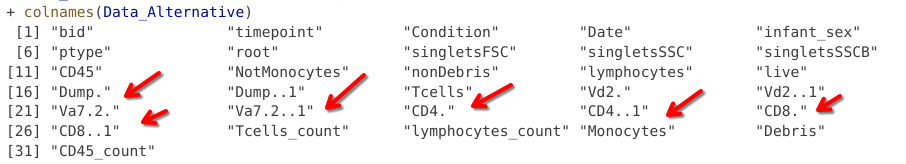
Since our dataset is stored as a .csv file, we will be using the read.csv() function from the utils package (included in our base R software installation) to read it into R. We will also use the colnames() function from last week to get a read-out of the column names.
 [1] "bid"               "timepoint"         "Condition"
 [4] "Date"              "infant_sex"        "ptype"
 [7] "root"              "singletsFSC"       "singletsSSC"
[10] "singletsSSCB"      "CD45"              "NotMonocytes"
[13] "nonDebris"         "lymphocytes"       "live"
[16] "Dump+"             "Dump-"             "Tcells"
[19] "Vd2+"              "Vd2-"              "Va7.2+"
[22] "Va7.2-"            "CD4+"              "CD4-"
[25] "CD8+"              "CD8-"              "Tcells_count"
[28] "lymphocytes_count" "Monocytes"         "Debris"
[31] "CD45_count"
.
As we look at the line of code, we now have enough context to decipher that the “file” argument is where we provide a file path to an individual file, but what does the “check.names” argument do?
Let’s see what happens to the column names when we set “check.names” argument to TRUE:
 [1] "bid"               "timepoint"         "Condition"
 [4] "Date"              "infant_sex"        "ptype"
 [7] "root"              "singletsFSC"       "singletsSSC"
[10] "singletsSSCB"      "CD45"              "NotMonocytes"
[13] "nonDebris"         "lymphocytes"       "live"
[16] "Dump."             "Dump..1"           "Tcells"
[19] "Vd2."              "Vd2..1"            "Va7.2."
[22] "Va7.2..1"          "CD4."              "CD4..1"
[25] "CD8."              "CD8..1"            "Tcells_count"
[28] "lymphocytes_count" "Monocytes"         "Debris"
[31] "CD45_count"
.
As we can see, any column name that contained a special character or a space was automatically converted over to R-approved syntax. However, this resulted in the loss of both +” and “-”, leaving us unable to determine whether we are looking at cells within or outside a particular gate.
.
Because of this, it is often better to rename columns individually after import, which we will learn how to do later today.
Following up with what we practiced last week, lets use the head() function to visualize the first few rows of data.
      bid timepoint Condition       Date infant_sex  ptype    root singletsFSC
1 INF0052         0      Ctrl 2025-07-26       Male HEU-hi 2098368     1894070
2 INF0100         0      Ctrl 2025-07-26       Male HEU-lo 2020184     1791890
3 INF0100         4      Ctrl 2025-07-26       Male HEU-lo 1155040     1033320
  singletsSSC singletsSSCB      CD45 NotMonocytes nonDebris lymphocytes
1     1666179      1537396 0.5952943    0.8820349 0.8627649   0.6420138
2     1697083      1579098 0.9106762    0.9052256 0.8602660   0.2145848
3      875465       845446 0.9705765    0.9845400 0.9578793   0.7403110
       live      Dump+     Dump-    Tcells        Vd2+      Vd2-     Va7.2+
1 0.9020581 0.21090996 0.6911482 0.2804264 0.008120361 0.9918796 0.01448070
2 0.8908981 0.06252775 0.8283703 0.6748298 0.007265620 0.9927344 0.01577499
3 0.8757665 0.20023803 0.6755285 0.6119129 0.004651313 0.9953487 0.01579402
     Va7.2-      CD4+      CD4-      CD8+       CD8- Tcells_count
1 0.9773989 0.6341164 0.3432825 0.2734826 0.06979990       164771
2 0.9769594 0.6119112 0.3650482 0.3357696 0.02927858       208241
3 0.9795547 0.6639621 0.3155925 0.2862104 0.02938209       371723
  lymphocytes_count  Monocytes     Debris CD45_count
1            587573 0.11796509 0.13723513     915203
2            308583 0.09477437 0.13973396    1438047
3            607477 0.01545999 0.04212072     820570
.
When working in Positron, we could have alternatively clicked on the little grid icon next to our created variable “Data” in the right secondary sidebar, which would have opened the data in our Editor window. From this same window, we can see it is stored as a “data.frame” object type.
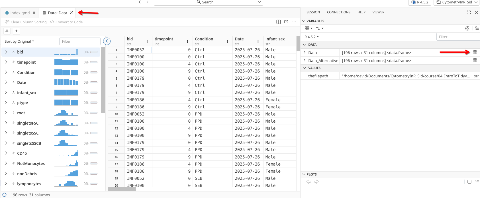
.
We could also achieve the same window to open using the View() function:
.
Wrapping up our brief recap of last week functions, we can check an objects type using both the class() and str() functions.
'data.frame':   196 obs. of  31 variables:
 $ bid              : chr  "INF0052" "INF0100" "INF0100" "INF0100" ...
 $ timepoint        : int  0 0 4 9 0 4 9 4 9 0 ...
 $ Condition        : chr  "Ctrl" "Ctrl" "Ctrl" "Ctrl" ...
 $ Date             : chr  "2025-07-26" "2025-07-26" "2025-07-26" "2025-07-26" ...
 $ infant_sex       : chr  "Male" "Male" "Male" "Male" ...
 $ ptype            : chr  "HEU-hi" "HEU-lo" "HEU-lo" "HEU-lo" ...
 $ root             : int  2098368 2020184 1155040 358624 1362216 1044808 1434840 972056 1521928 2363512 ...
 $ singletsFSC      : int  1894070 1791890 1033320 328624 1206309 917398 1265022 875707 1359574 2136616 ...
 $ singletsSSC      : int  1666179 1697083 875465 289327 1032946 735579 988445 767323 1175755 1875394 ...
 $ singletsSSCB     : int  1537396 1579098 845446 276289 982736 685592 940454 718000 1097478 1732620 ...
 $ CD45             : num  0.595 0.911 0.971 0.982 0.957 ...
 $ NotMonocytes     : num  0.882 0.905 0.985 0.986 0.956 ...
 $ nonDebris        : num  0.863 0.86 0.958 0.941 0.841 ...
 $ lymphocytes      : num  0.642 0.215 0.74 0.651 0.705 ...
 $ live             : num  0.902 0.891 0.876 0.915 0.895 ...
 $ Dump+            : num  0.2109 0.0625 0.2002 0.2147 0.3383 ...
 $ Dump-            : num  0.691 0.828 0.676 0.701 0.557 ...
 $ Tcells           : num  0.28 0.675 0.612 0.631 0.44 ...
 $ Vd2+             : num  0.00812 0.00727 0.00465 0.01135 0.00475 ...
 $ Vd2-             : num  0.992 0.993 0.995 0.989 0.995 ...
 $ Va7.2+           : num  0.0145 0.0158 0.0158 0.017 0.0133 ...
 $ Va7.2-           : num  0.977 0.977 0.98 0.972 0.982 ...
 $ CD4+             : num  0.634 0.612 0.664 0.438 0.739 ...
 $ CD4-             : num  0.343 0.365 0.316 0.534 0.243 ...
 $ CD8+             : num  0.273 0.336 0.286 0.486 0.195 ...
 $ CD8-             : num  0.0698 0.0293 0.0294 0.0476 0.0476 ...
 $ Tcells_count     : int  164771 208241 371723 111552 291777 271870 487937 220634 415867 184930 ...
 $ lymphocytes_count: int  587573 308583 607477 176662 663667 510730 726238 451047 710964 652155 ...
 $ Monocytes        : num  0.118 0.0948 0.0155 0.0145 0.0444 ...
 $ Debris           : num  0.1372 0.1397 0.0421 0.0587 0.1592 ...
 $ CD45_count       : int  915203 1438047 820570 271304 940733 675857 921660 701657 1066884 1017713 ...
data.frame
.
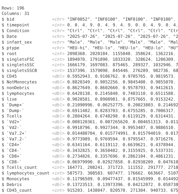
Or alternatively using the new-to-us glimpse() function
Checkpoint 1
This however returns an error. Any idea why this might be occuring?
Checkpoint 2
How would we locate a package a not-yet-loaded function is within?

.
From the list of search matches (in the right secondary sidebar), it looks likely that the glimpse() function in the dplyr package was the one we were looking for. This is one the main tidyverse packages we will be using throughout the course. Let’s attach it to our environment via the library() call first and try running glimpse() again.
Rows: 196
Columns: 31
$ bid               <chr> "INF0052", "INF0100", "INF0100", "INF0100", "INF0179…
$ timepoint         <int> 0, 0, 4, 9, 0, 4, 9, 4, 9, 0, 0, 4, 9, 0, 4, 9, 4, 9…
$ Condition         <chr> "Ctrl", "Ctrl", "Ctrl", "Ctrl", "Ctrl", "Ctrl", "Ctr…
$ Date              <chr> "2025-07-26", "2025-07-26", "2025-07-26", "2025-07-2…
$ infant_sex        <chr> "Male", "Male", "Male", "Male", "Male", "Male", "Mal…
$ ptype             <chr> "HEU-hi", "HEU-lo", "HEU-lo", "HEU-lo", "HU", "HU", …
$ root              <int> 2098368, 2020184, 1155040, 358624, 1362216, 1044808,…
$ singletsFSC       <int> 1894070, 1791890, 1033320, 328624, 1206309, 917398, …
$ singletsSSC       <int> 1666179, 1697083, 875465, 289327, 1032946, 735579, 9…
$ singletsSSCB      <int> 1537396, 1579098, 845446, 276289, 982736, 685592, 94…
$ CD45              <dbl> 0.5952943, 0.9106762, 0.9705765, 0.9819573, 0.957259…
$ NotMonocytes      <dbl> 0.8820349, 0.9052256, 0.9845400, 0.9855070, 0.955627…
$ nonDebris         <dbl> 0.8627649, 0.8602660, 0.9578793, 0.9412615, 0.840783…
$ lymphocytes       <dbl> 0.6420138, 0.2145848, 0.7403110, 0.6511588, 0.705478…
$ live              <dbl> 0.9020581, 0.8908981, 0.8757665, 0.9153242, 0.895214…
$ `Dump+`           <dbl> 0.21090996, 0.06252775, 0.20023803, 0.21469246, 0.33…
$ `Dump-`           <dbl> 0.6911482, 0.8283703, 0.6755285, 0.7006317, 0.556895…
$ Tcells            <dbl> 0.2804264, 0.6748298, 0.6119129, 0.6314431, 0.439643…
$ `Vd2+`            <dbl> 0.008120361, 0.007265620, 0.004651313, 0.011348967, …
$ `Vd2-`            <dbl> 0.9918796, 0.9927344, 0.9953487, 0.9886510, 0.995246…
$ `Va7.2+`          <dbl> 0.014480704, 0.015774991, 0.015794019, 0.017023451, …
$ `Va7.2-`          <dbl> 0.9773989, 0.9769594, 0.9795547, 0.9716276, 0.981924…
$ `CD4+`            <dbl> 0.6341164, 0.6119112, 0.6639621, 0.4378944, 0.739256…
$ `CD4-`            <dbl> 0.3432825, 0.3650482, 0.3155925, 0.5337331, 0.242668…
$ `CD8+`            <dbl> 0.2734826, 0.3357696, 0.2862104, 0.4861231, 0.195063…
$ `CD8-`            <dbl> 0.06979990, 0.02927858, 0.02938209, 0.04761008, 0.04…
$ Tcells_count      <int> 164771, 208241, 371723, 111552, 291777, 271870, 4879…
$ lymphocytes_count <int> 587573, 308583, 607477, 176662, 663667, 510730, 7262…
$ Monocytes         <dbl> 0.11796509, 0.09477437, 0.01545999, 0.01449297, 0.04…
$ Debris            <dbl> 0.13723513, 0.13973396, 0.04212072, 0.05873854, 0.15…
$ CD45_count        <int> 915203, 1438047, 820570, 271304, 940733, 675857, 921…
.
We notice that while similar to the str() output, glimpse() handles spacing a little differently, and includes the dimensions at the top. However, we can also retrieve the dimensions directly using the dim() function (which maintains the row followed by column position convention of base R (ex. [196,31]))
Column value type
.
As we saw last week, functions often need values that match a certain type (the paintbrush needing paint analogy). As we inspect the columns of Data, we can notice some of the columns contain values within that are character (ie. “char”) values. Others appear to contain numeric values (which are subtyped as either double (“ie. dbl”) or integer (ie. “int”)). At first glance, we do not appear to have any logical (ie. TRUE or FALSE) columns in this dataset.
.
If we were trying to verify type of values contained within a data.frame column, we could employ several similarly-named functions (is.character(), is.numeric() or is.logical()) to check
.
For numeric columns using the is.numeric() function, we can also be subtype specific using either is.integer() or is.double().
Reminder
As we observed last week with keywords, column names that contain special characters like $ or spaces will need to be surrounded with tick marks in order for the function to be able to run.
select (Columns)
.
Now that we have read in our data, and have a general picture of the structure and contents, lets start learning the main dplyr functions we will be using throughout the course. To do this, lets go ahead and attach dplyr to our local environment via the library() call.
.
We will start with the select() function. It is used to “select” a column from a data.frame type object. In the simplest usage, we provide the name of our data.frame variable/object as the first argument after the opening parenthesis. This is then followed by the name of the column we want to select as the second argument (let’s place around the “” around the column name for now)
          Date
1   2025-07-26
2   2025-07-26
3   2025-07-26
4   2025-07-26
5   2025-07-26
6   2025-07-26
7   2025-07-26
8   2025-07-26
9   2025-07-26
10  2025-07-26
11  2025-07-26
12  2025-07-26
13  2025-07-26
14  2025-07-26
15  2025-07-26
16  2025-07-26
17  2025-07-26
18  2025-07-26
19  2025-07-26
20  2025-07-26
21  2025-07-26
22  2025-07-26
23  2025-07-26
24  2025-07-26
25  2025-07-26
26  2025-07-26
27  2025-07-29
28  2025-07-29
29  2025-07-29
30  2025-07-29
31  2025-07-29
32  2025-07-29
33  2025-07-29
34  2025-07-29
35  2025-07-29
36  2025-07-29
37  2025-07-29
38  2025-07-29
39  2025-07-29
40  2025-07-29
41  2025-07-29
42  2025-07-29
43  2025-07-29
44  2025-07-29
45  2025-07-29
46  2025-07-29
47  2025-07-29
48  2025-07-29
49  2025-07-31
50  2025-07-31
51  2025-07-31
52  2025-07-31
53  2025-07-31
54  2025-07-31
55  2025-07-31
56  2025-07-31
57  2025-07-31
58  2025-07-31
59  2025-07-31
60  2025-07-31
61  2025-07-31
62  2025-07-31
63  2025-07-31
64  2025-07-31
65  2025-07-31
66  2025-07-31
67  2025-07-31
68  2025-07-31
69  2025-07-31
70  2025-07-31
71  2025-07-31
72  2025-07-31
73  2025-07-31
74  2025-07-31
75  2025-07-31
76  2025-08-05
77  2025-08-05
78  2025-08-05
79  2025-08-05
80  2025-08-05
81  2025-08-05
82  2025-08-05
83  2025-08-05
84  2025-08-05
85  2025-08-05
86  2025-08-05
87  2025-08-05
88  2025-08-05
89  2025-08-05
90  2025-08-05
91  2025-08-05
92  2025-08-05
93  2025-08-05
94  2025-08-05
95  2025-08-05
96  2025-08-05
97  2025-08-05
98  2025-08-05
99  2025-08-07
100 2025-08-07
101 2025-08-07
102 2025-08-07
103 2025-08-07
104 2025-08-07
105 2025-08-07
106 2025-08-07
107 2025-08-07
108 2025-08-07
109 2025-08-07
110 2025-08-07
111 2025-08-07
112 2025-08-07
113 2025-08-07
114 2025-08-07
115 2025-08-07
116 2025-08-07
117 2025-08-07
118 2025-08-07
119 2025-08-07
120 2025-08-07
121 2025-08-07
122 2025-08-07
123 2025-08-07
124 2025-08-07
125 2025-08-22
126 2025-08-22
127 2025-08-22
128 2025-08-22
129 2025-08-22
130 2025-08-22
131 2025-08-22
132 2025-08-22
133 2025-08-22
134 2025-08-22
135 2025-08-22
136 2025-08-22
137 2025-08-22
138 2025-08-22
139 2025-08-22
140 2025-08-22
141 2025-08-22
142 2025-08-22
143 2025-08-22
144 2025-08-22
145 2025-08-22
146 2025-08-22
147 2025-08-22
148 2025-08-22
149 2025-08-22
150 2025-08-22
151 2025-08-22
152 2025-08-28
153 2025-08-28
154 2025-08-28
155 2025-08-28
156 2025-08-28
157 2025-08-28
158 2025-08-28
159 2025-08-28
160 2025-08-28
161 2025-08-28
162 2025-08-28
163 2025-08-28
164 2025-08-28
165 2025-08-28
166 2025-08-28
167 2025-08-28
168 2025-08-28
169 2025-08-28
170 2025-08-28
171 2025-08-28
172 2025-08-28
173 2025-08-28
174 2025-08-28
175 2025-08-28
176 2025-08-28
177 2025-08-28
178 2025-08-28
179 2025-08-30
180 2025-08-30
181 2025-08-30
182 2025-08-30
183 2025-08-30
184 2025-08-30
185 2025-08-30
186 2025-08-30
187 2025-08-30
188 2025-08-30
189 2025-08-30
190 2025-08-30
191 2025-08-30
192 2025-08-30
193 2025-08-30
194 2025-08-30
195 2025-08-30
196 2025-08-30
.
This results in the column being selected, resulting in the new object containing only that subsetted out column from the original Data object.
Pipe Operators
.
While the above line of code works to select a column, when you encounter select() out in the wild, it will more often be in a line of code that looks like this:
          Date
1   2025-07-26
2   2025-07-26
3   2025-07-26
4   2025-07-26
5   2025-07-26
6   2025-07-26
7   2025-07-26
8   2025-07-26
9   2025-07-26
10  2025-07-26
11  2025-07-26
12  2025-07-26
13  2025-07-26
14  2025-07-26
15  2025-07-26
16  2025-07-26
17  2025-07-26
18  2025-07-26
19  2025-07-26
20  2025-07-26
21  2025-07-26
22  2025-07-26
23  2025-07-26
24  2025-07-26
25  2025-07-26
26  2025-07-26
27  2025-07-29
28  2025-07-29
29  2025-07-29
30  2025-07-29
31  2025-07-29
32  2025-07-29
33  2025-07-29
34  2025-07-29
35  2025-07-29
36  2025-07-29
37  2025-07-29
38  2025-07-29
39  2025-07-29
40  2025-07-29
41  2025-07-29
42  2025-07-29
43  2025-07-29
44  2025-07-29
45  2025-07-29
46  2025-07-29
47  2025-07-29
48  2025-07-29
49  2025-07-31
50  2025-07-31
51  2025-07-31
52  2025-07-31
53  2025-07-31
54  2025-07-31
55  2025-07-31
56  2025-07-31
57  2025-07-31
58  2025-07-31
59  2025-07-31
60  2025-07-31
61  2025-07-31
62  2025-07-31
63  2025-07-31
64  2025-07-31
65  2025-07-31
66  2025-07-31
67  2025-07-31
68  2025-07-31
69  2025-07-31
70  2025-07-31
71  2025-07-31
72  2025-07-31
73  2025-07-31
74  2025-07-31
75  2025-07-31
76  2025-08-05
77  2025-08-05
78  2025-08-05
79  2025-08-05
80  2025-08-05
81  2025-08-05
82  2025-08-05
83  2025-08-05
84  2025-08-05
85  2025-08-05
86  2025-08-05
87  2025-08-05
88  2025-08-05
89  2025-08-05
90  2025-08-05
91  2025-08-05
92  2025-08-05
93  2025-08-05
94  2025-08-05
95  2025-08-05
96  2025-08-05
97  2025-08-05
98  2025-08-05
99  2025-08-07
100 2025-08-07
101 2025-08-07
102 2025-08-07
103 2025-08-07
104 2025-08-07
105 2025-08-07
106 2025-08-07
107 2025-08-07
108 2025-08-07
109 2025-08-07
110 2025-08-07
111 2025-08-07
112 2025-08-07
113 2025-08-07
114 2025-08-07
115 2025-08-07
116 2025-08-07
117 2025-08-07
118 2025-08-07
119 2025-08-07
120 2025-08-07
121 2025-08-07
122 2025-08-07
123 2025-08-07
124 2025-08-07
125 2025-08-22
126 2025-08-22
127 2025-08-22
128 2025-08-22
129 2025-08-22
130 2025-08-22
131 2025-08-22
132 2025-08-22
133 2025-08-22
134 2025-08-22
135 2025-08-22
136 2025-08-22
137 2025-08-22
138 2025-08-22
139 2025-08-22
140 2025-08-22
141 2025-08-22
142 2025-08-22
143 2025-08-22
144 2025-08-22
145 2025-08-22
146 2025-08-22
147 2025-08-22
148 2025-08-22
149 2025-08-22
150 2025-08-22
151 2025-08-22
152 2025-08-28
153 2025-08-28
154 2025-08-28
155 2025-08-28
156 2025-08-28
157 2025-08-28
158 2025-08-28
159 2025-08-28
160 2025-08-28
161 2025-08-28
162 2025-08-28
163 2025-08-28
164 2025-08-28
165 2025-08-28
166 2025-08-28
167 2025-08-28
168 2025-08-28
169 2025-08-28
170 2025-08-28
171 2025-08-28
172 2025-08-28
173 2025-08-28
174 2025-08-28
175 2025-08-28
176 2025-08-28
177 2025-08-28
178 2025-08-28
179 2025-08-30
180 2025-08-30
181 2025-08-30
182 2025-08-30
183 2025-08-30
184 2025-08-30
185 2025-08-30
186 2025-08-30
187 2025-08-30
188 2025-08-30
189 2025-08-30
190 2025-08-30
191 2025-08-30
192 2025-08-30
193 2025-08-30
194 2025-08-30
195 2025-08-30
196 2025-08-30
.
… “What in the world is that thing |> ?” …
.
Glad you asked! An useful feature of the tidyverse packages is their use of pipes (either the original magrittr package’s “%>%” or base R version >4.1.0's “|>”“), usually appearing like this:
.
… “How do we interpret/read that line of code?” …
.
Let’s break it down, starting off just to the right of the assignment arrow (<-) with our data.frame “Data”.
.
We then proceed to read to the right, adding in our pipe operator. The pipe essentially serves as an intermediate passing the contents of data onward to the subsequent function.
.
In our case, this subsequent function is the select() function, which will select a particular column from the available data. When using the pipe, the first argument slot we saw for “select(Data,”Date”)” is occupied by the contents Data that are being passed by the pipe.
.
To complete the transfer, we provide the desired column name to select() to act on (“Date” in this case)
.
In summary, contents of Data are passed to the pipe, and select runs on those contents to select the Date column
          Date
1   2025-07-26
2   2025-07-26
3   2025-07-26
4   2025-07-26
5   2025-07-26
6   2025-07-26
7   2025-07-26
8   2025-07-26
9   2025-07-26
10  2025-07-26
11  2025-07-26
12  2025-07-26
13  2025-07-26
14  2025-07-26
15  2025-07-26
16  2025-07-26
17  2025-07-26
18  2025-07-26
19  2025-07-26
20  2025-07-26
21  2025-07-26
22  2025-07-26
23  2025-07-26
24  2025-07-26
25  2025-07-26
26  2025-07-26
27  2025-07-29
28  2025-07-29
29  2025-07-29
30  2025-07-29
31  2025-07-29
32  2025-07-29
33  2025-07-29
34  2025-07-29
35  2025-07-29
36  2025-07-29
37  2025-07-29
38  2025-07-29
39  2025-07-29
40  2025-07-29
41  2025-07-29
42  2025-07-29
43  2025-07-29
44  2025-07-29
45  2025-07-29
46  2025-07-29
47  2025-07-29
48  2025-07-29
49  2025-07-31
50  2025-07-31
51  2025-07-31
52  2025-07-31
53  2025-07-31
54  2025-07-31
55  2025-07-31
56  2025-07-31
57  2025-07-31
58  2025-07-31
59  2025-07-31
60  2025-07-31
61  2025-07-31
62  2025-07-31
63  2025-07-31
64  2025-07-31
65  2025-07-31
66  2025-07-31
67  2025-07-31
68  2025-07-31
69  2025-07-31
70  2025-07-31
71  2025-07-31
72  2025-07-31
73  2025-07-31
74  2025-07-31
75  2025-07-31
76  2025-08-05
77  2025-08-05
78  2025-08-05
79  2025-08-05
80  2025-08-05
81  2025-08-05
82  2025-08-05
83  2025-08-05
84  2025-08-05
85  2025-08-05
86  2025-08-05
87  2025-08-05
88  2025-08-05
89  2025-08-05
90  2025-08-05
91  2025-08-05
92  2025-08-05
93  2025-08-05
94  2025-08-05
95  2025-08-05
96  2025-08-05
97  2025-08-05
98  2025-08-05
99  2025-08-07
100 2025-08-07
101 2025-08-07
102 2025-08-07
103 2025-08-07
104 2025-08-07
105 2025-08-07
106 2025-08-07
107 2025-08-07
108 2025-08-07
109 2025-08-07
110 2025-08-07
111 2025-08-07
112 2025-08-07
113 2025-08-07
114 2025-08-07
115 2025-08-07
116 2025-08-07
117 2025-08-07
118 2025-08-07
119 2025-08-07
120 2025-08-07
121 2025-08-07
122 2025-08-07
123 2025-08-07
124 2025-08-07
125 2025-08-22
126 2025-08-22
127 2025-08-22
128 2025-08-22
129 2025-08-22
130 2025-08-22
131 2025-08-22
132 2025-08-22
133 2025-08-22
134 2025-08-22
135 2025-08-22
136 2025-08-22
137 2025-08-22
138 2025-08-22
139 2025-08-22
140 2025-08-22
141 2025-08-22
142 2025-08-22
143 2025-08-22
144 2025-08-22
145 2025-08-22
146 2025-08-22
147 2025-08-22
148 2025-08-22
149 2025-08-22
150 2025-08-22
151 2025-08-22
152 2025-08-28
153 2025-08-28
154 2025-08-28
155 2025-08-28
156 2025-08-28
157 2025-08-28
158 2025-08-28
159 2025-08-28
160 2025-08-28
161 2025-08-28
162 2025-08-28
163 2025-08-28
164 2025-08-28
165 2025-08-28
166 2025-08-28
167 2025-08-28
168 2025-08-28
169 2025-08-28
170 2025-08-28
171 2025-08-28
172 2025-08-28
173 2025-08-28
174 2025-08-28
175 2025-08-28
176 2025-08-28
177 2025-08-28
178 2025-08-28
179 2025-08-30
180 2025-08-30
181 2025-08-30
182 2025-08-30
183 2025-08-30
184 2025-08-30
185 2025-08-30
186 2025-08-30
187 2025-08-30
188 2025-08-30
189 2025-08-30
190 2025-08-30
191 2025-08-30
192 2025-08-30
193 2025-08-30
194 2025-08-30
195 2025-08-30
196 2025-08-30
.
One of the main advantages for using pipes, is they can be linked together, passing resulting objects of one operation on to the next pipe and subsequent function. We can see this in operation in the example below where we hand off the isolated “Date” column to the nrow() function to determine number of rows. We will use pipes throughout the course, so you will gradually gain familiarity as you encounter them.
.
For those with prior R experience, you will be more familiar with the older magrittr %>% pipe. The base R |> pipe operator was introduced starting with R version 4.1.0. While mostly interchangeable, they have a few nuances that come into play for more advance use cases. You are welcome to use whichever you prefer (my current preference is |> as it’s one less key to press).
R Quirks
Odd R Behavior # 1
While we used “” around the column name in our previous example, unlike what we encountered with install.packages() when we forget to include quotation marks, select() still retrieves the correct column despite Date not being an environment variable:
.
The reasons for this Odd R behaviour are nuanced and for another day. For now, think of it as dplyr R package is picking up the slack, and using context to infer it’s a column name and not an environmental variable/object.
Selecting multiple columns
.
Since we are able to select one column, can we select multiple (similar to a [Data[,2:5]] approach in base R)? We can, and they can be positioned anywhere within the data.frame:
      bid timepoint Condition    Tcells      CD8+      CD4+
1 INF0052         0      Ctrl 0.2804264 0.2734826 0.6341164
2 INF0100         0      Ctrl 0.6748298 0.3357696 0.6119112
3 INF0100         4      Ctrl 0.6119129 0.2862104 0.6639621
4 INF0100         9      Ctrl 0.6314431 0.4861231 0.4378944
5 INF0179         0      Ctrl 0.4396437 0.1950634 0.7392563
.
You will notice that the order in which we selected the columns will dictate their position in the subsetted data.frame object:
      bid    Tcells      CD8+      CD4+ timepoint Condition
1 INF0052 0.2804264 0.2734826 0.6341164         0      Ctrl
2 INF0100 0.6748298 0.3357696 0.6119112         0      Ctrl
3 INF0100 0.6119129 0.2862104 0.6639621         4      Ctrl
4 INF0100 0.6314431 0.4861231 0.4378944         9      Ctrl
5 INF0179 0.4396437 0.1950634 0.7392563         0      Ctrl
relocate
.
Alternatively, we occasionally want to move one column. While we could respecify the location using select(), specifying the names of all the other columns out in a line of code to just to rearrange one does not sound like a good use of time. For this reason, the second dplyr function we will be learning is the relocate() function.
.
Looking at our Data object, let’s say we wanted to move the Tcells column from its current location to the second column position (right after the bid column). The line of code to do so would look like:
      bid    Tcells timepoint Condition       Date infant_sex  ptype    root
1 INF0052 0.2804264         0      Ctrl 2025-07-26       Male HEU-hi 2098368
2 INF0100 0.6748298         0      Ctrl 2025-07-26       Male HEU-lo 2020184
3 INF0100 0.6119129         4      Ctrl 2025-07-26       Male HEU-lo 1155040
4 INF0100 0.6314431         9      Ctrl 2025-07-26       Male HEU-lo  358624
5 INF0179 0.4396437         0      Ctrl 2025-07-26       Male     HU 1362216
  singletsFSC singletsSSC singletsSSCB      CD45 NotMonocytes nonDebris
1     1894070     1666179      1537396 0.5952943    0.8820349 0.8627649
2     1791890     1697083      1579098 0.9106762    0.9052256 0.8602660
3     1033320      875465       845446 0.9705765    0.9845400 0.9578793
4      328624      289327       276289 0.9819573    0.9855070 0.9412615
5     1206309     1032946       982736 0.9572591    0.9556272 0.8407837
  lymphocytes      live      Dump+     Dump-        Vd2+      Vd2-     Va7.2+
1   0.6420138 0.9020581 0.21090996 0.6911482 0.008120361 0.9918796 0.01448070
2   0.2145848 0.8908981 0.06252775 0.8283703 0.007265620 0.9927344 0.01577499
3   0.7403110 0.8757665 0.20023803 0.6755285 0.004651313 0.9953487 0.01579402
4   0.6511588 0.9153242 0.21469246 0.7006317 0.011348967 0.9886510 0.01702345
5   0.7054786 0.8952140 0.33831877 0.5568953 0.004753630 0.9952464 0.01332182
     Va7.2-      CD4+      CD4-      CD8+       CD8- Tcells_count
1 0.9773989 0.6341164 0.3432825 0.2734826 0.06979990       164771
2 0.9769594 0.6119112 0.3650482 0.3357696 0.02927858       208241
3 0.9795547 0.6639621 0.3155925 0.2862104 0.02938209       371723
4 0.9716276 0.4378944 0.5337331 0.4861231 0.04761008       111552
5 0.9819246 0.7392563 0.2426682 0.1950634 0.04760485       291777
  lymphocytes_count  Monocytes     Debris CD45_count
1            587573 0.11796509 0.13723513     915203
2            308583 0.09477437 0.13973396    1438047
3            607477 0.01545999 0.04212072     820570
4            176662 0.01449297 0.05873854     271304
5 663667 0.04437285 0.15921627 940733.
Similar to what we saw with select(), this approach can also be used for more than 1 column:
      bid    Tcells  Monocytes timepoint Condition       Date infant_sex  ptype
1 INF0052 0.2804264 0.11796509         0      Ctrl 2025-07-26       Male HEU-hi
2 INF0100 0.6748298 0.09477437         0      Ctrl 2025-07-26       Male HEU-lo
3 INF0100 0.6119129 0.01545999         4      Ctrl 2025-07-26       Male HEU-lo
4 INF0100 0.6314431 0.01449297         9      Ctrl 2025-07-26       Male HEU-lo
5 INF0179 0.4396437 0.04437285         0      Ctrl 2025-07-26       Male     HU
     root singletsFSC singletsSSC singletsSSCB      CD45 NotMonocytes nonDebris
1 2098368     1894070     1666179      1537396 0.5952943    0.8820349 0.8627649
2 2020184     1791890     1697083      1579098 0.9106762    0.9052256 0.8602660
3 1155040     1033320      875465       845446 0.9705765    0.9845400 0.9578793
4  358624      328624      289327       276289 0.9819573    0.9855070 0.9412615
5 1362216     1206309     1032946       982736 0.9572591    0.9556272 0.8407837
  lymphocytes      live      Dump+     Dump-        Vd2+      Vd2-     Va7.2+
1   0.6420138 0.9020581 0.21090996 0.6911482 0.008120361 0.9918796 0.01448070
2   0.2145848 0.8908981 0.06252775 0.8283703 0.007265620 0.9927344 0.01577499
3   0.7403110 0.8757665 0.20023803 0.6755285 0.004651313 0.9953487 0.01579402
4   0.6511588 0.9153242 0.21469246 0.7006317 0.011348967 0.9886510 0.01702345
5   0.7054786 0.8952140 0.33831877 0.5568953 0.004753630 0.9952464 0.01332182
     Va7.2-      CD4+      CD4-      CD8+       CD8- Tcells_count
1 0.9773989 0.6341164 0.3432825 0.2734826 0.06979990       164771
2 0.9769594 0.6119112 0.3650482 0.3357696 0.02927858       208241
3 0.9795547 0.6639621 0.3155925 0.2862104 0.02938209       371723
4 0.9716276 0.4378944 0.5337331 0.4861231 0.04761008       111552
5 0.9819246 0.7392563 0.2426682 0.1950634 0.04760485       291777
  lymphocytes_count     Debris CD45_count
1            587573 0.13723513     915203
2            308583 0.13973396    1438047
3            607477 0.04212072     820570
4            176662 0.05873854     271304
5 663667 0.15921627 940733.
We can also modify the argument so that columns are placed before a certain column
      bid timepoint Condition    Tcells       Date infant_sex  ptype    root
1 INF0052         0      Ctrl 0.2804264 2025-07-26       Male HEU-hi 2098368
2 INF0100         0      Ctrl 0.6748298 2025-07-26       Male HEU-lo 2020184
3 INF0100         4      Ctrl 0.6119129 2025-07-26       Male HEU-lo 1155040
4 INF0100         9      Ctrl 0.6314431 2025-07-26       Male HEU-lo  358624
5 INF0179         0      Ctrl 0.4396437 2025-07-26       Male     HU 1362216
  singletsFSC singletsSSC singletsSSCB      CD45 NotMonocytes nonDebris
1     1894070     1666179      1537396 0.5952943    0.8820349 0.8627649
2     1791890     1697083      1579098 0.9106762    0.9052256 0.8602660
3     1033320      875465       845446 0.9705765    0.9845400 0.9578793
4      328624      289327       276289 0.9819573    0.9855070 0.9412615
5     1206309     1032946       982736 0.9572591    0.9556272 0.8407837
  lymphocytes      live      Dump+     Dump-        Vd2+      Vd2-     Va7.2+
1   0.6420138 0.9020581 0.21090996 0.6911482 0.008120361 0.9918796 0.01448070
2   0.2145848 0.8908981 0.06252775 0.8283703 0.007265620 0.9927344 0.01577499
3   0.7403110 0.8757665 0.20023803 0.6755285 0.004651313 0.9953487 0.01579402
4   0.6511588 0.9153242 0.21469246 0.7006317 0.011348967 0.9886510 0.01702345
5   0.7054786 0.8952140 0.33831877 0.5568953 0.004753630 0.9952464 0.01332182
     Va7.2-      CD4+      CD4-      CD8+       CD8- Tcells_count
1 0.9773989 0.6341164 0.3432825 0.2734826 0.06979990       164771
2 0.9769594 0.6119112 0.3650482 0.3357696 0.02927858       208241
3 0.9795547 0.6639621 0.3155925 0.2862104 0.02938209       371723
4 0.9716276 0.4378944 0.5337331 0.4861231 0.04761008       111552
5 0.9819246 0.7392563 0.2426682 0.1950634 0.04760485       291777
  lymphocytes_count  Monocytes     Debris CD45_count
1            587573 0.11796509 0.13723513     915203
2            308583 0.09477437 0.13973396    1438047
3            607477 0.01545999 0.04212072     820570
4            176662 0.01449297 0.05873854     271304
5 663667 0.04437285 0.15921627 940733.
And as we might suspect, we could specify a column index location rather than using a column name.
        Date     bid timepoint Condition infant_sex  ptype    root singletsFSC
1 2025-07-26 INF0052         0      Ctrl       Male HEU-hi 2098368     1894070
2 2025-07-26 INF0100         0      Ctrl       Male HEU-lo 2020184     1791890
3 2025-07-26 INF0100         4      Ctrl       Male HEU-lo 1155040     1033320
4 2025-07-26 INF0100         9      Ctrl       Male HEU-lo  358624      328624
5 2025-07-26 INF0179         0      Ctrl       Male     HU 1362216     1206309
  singletsSSC singletsSSCB      CD45 NotMonocytes nonDebris lymphocytes
1     1666179      1537396 0.5952943    0.8820349 0.8627649   0.6420138
2     1697083      1579098 0.9106762    0.9052256 0.8602660   0.2145848
3      875465       845446 0.9705765    0.9845400 0.9578793   0.7403110
4      289327       276289 0.9819573    0.9855070 0.9412615   0.6511588
5     1032946       982736 0.9572591    0.9556272 0.8407837   0.7054786
       live      Dump+     Dump-    Tcells        Vd2+      Vd2-     Va7.2+
1 0.9020581 0.21090996 0.6911482 0.2804264 0.008120361 0.9918796 0.01448070
2 0.8908981 0.06252775 0.8283703 0.6748298 0.007265620 0.9927344 0.01577499
3 0.8757665 0.20023803 0.6755285 0.6119129 0.004651313 0.9953487 0.01579402
4 0.9153242 0.21469246 0.7006317 0.6314431 0.011348967 0.9886510 0.01702345
5 0.8952140 0.33831877 0.5568953 0.4396437 0.004753630 0.9952464 0.01332182
     Va7.2-      CD4+      CD4-      CD8+       CD8- Tcells_count
1 0.9773989 0.6341164 0.3432825 0.2734826 0.06979990       164771
2 0.9769594 0.6119112 0.3650482 0.3357696 0.02927858       208241
3 0.9795547 0.6639621 0.3155925 0.2862104 0.02938209       371723
4 0.9716276 0.4378944 0.5337331 0.4861231 0.04761008       111552
5 0.9819246 0.7392563 0.2426682 0.1950634 0.04760485       291777
  lymphocytes_count  Monocytes     Debris CD45_count
1            587573 0.11796509 0.13723513     915203
2            308583 0.09477437 0.13973396    1438047
3            607477 0.01545999 0.04212072     820570
4            176662 0.01449297 0.05873854     271304
5 663667 0.04437285 0.15921627 940733rename
.
At this point, we are able to both move and select particular columns, allowing us to rearrange and subset a larger data.frame object however we want it to appear. However, as we encountered, some of the names contain special characters and spaces, requiring use of tick marks (``) to avoid issues. How can we change a column name?
.
In base R, we could change individual column names by assigning a new value with the assignment arrow to the corresponding column name index. For example, looking at our Subset object, wen could rename CD8+ as follows:
.
With the tidyverse, we can use the rename() function which removes the need to look up the column index number. The way we write the argument is placing within the parenthesis the old name to the right of the equals sign, with the new name to the left
.
If we wanted to rename multiple column names at once, we would just need to include a comma between the individual rename arguments within the parenthesis.
pull
.
Sometimes, we may want to retrieve individual values present in a column, to use within either a vector or a list. We can do this using the pull() function, which will retrieve the column contents and strip the column formatting
.
This can be useful when we are doing data exploration, and trying to determine how many unique variants might be present. For example, if we wanted to see what days individual samples were acquired, we could pull() the data and pass it to the unique() function:
filter (Rows)
.
So far, we have been working with dplyr functions primarily used when working with and subsetting columns (including select(), pull(), rename() and relocate()). What if we wanted to work with rows of a data.frame? This is where the filter() function is used.
.
The Condition column in this Dataset appears to be indicating whether the samples were stimulated. Let’s see how many unique values are contained within that column
.
In the case of this dataset, looks like the .fcs files where treated with either left alone, treated with PPD (Purified Protein Derrivative) or SEB. What if we wanted to subset only those treated with PPD?
.
Within filter(), we would specify the column name as the first argument, and ask that only values equal to (==) “PPD” be returned. Notice in this case, “” are needed, as we are asking for a matching character value.
      bid timepoint Condition       Date infant_sex  ptype    root singletsFSC
1 INF0052         0       PPD 2025-07-26       Male HEU-hi 2363512     2136616
2 INF0100         0       PPD 2025-07-26       Male HEU-lo 2049112     1821676
3 INF0100         4       PPD 2025-07-26       Male HEU-lo 1063496      946587
4 INF0100         9       PPD 2025-07-26       Male HEU-lo  788368      714198
5 INF0179         0       PPD 2025-07-26       Male     HU 1380336     1242311
  singletsSSC singletsSSCB      CD45 NotMonocytes nonDebris lymphocytes
1     1875394      1732620 0.5873838    0.8619837 0.8429685   0.6408044
2     1717636      1597085 0.9063081    0.9251961 0.8771889   0.2174284
3      796056       767297 0.9709891    0.9848719 0.9556049   0.7313503
4      626387       600011 0.9822803    0.9842139 0.8123041   0.6223228
5     1047081      1000877 0.9470275    0.9575685 0.9134438   0.6996502
       live      Dump+     Dump-    Tcells        Vd2+      Vd2-     Va7.2+
1 0.9009254 0.20743228 0.6934931 0.2835676 0.007408209 0.9925918 0.01507057
2 0.8929673 0.06181426 0.8311531 0.6735798 0.007137230 0.9928628 0.01671801
3 0.8782307 0.20727202 0.6709587 0.5989873 0.005254643 0.9947454 0.01609790
4 0.9566639 0.23164587 0.7250180 0.6489405 0.011935922 0.9880641 0.01855298
5 0.8856898 0.33186111 0.5538287 0.4441538 0.004382972 0.9956170 0.01297237
     Va7.2-      CD4+      CD4-      CD8+       CD8- Tcells_count
1 0.9775212 0.6340345 0.3434867 0.2744119 0.06907479       184930
2 0.9761448 0.6145707 0.3615741 0.3312279 0.03034620       211987
3 0.9786475 0.6559480 0.3226994 0.2912084 0.03149109       326378
4 0.9695111 0.4306889 0.5388222 0.4908558 0.04796636       238021
5 0.9826447 0.7499194 0.2327253 0.1850897 0.04763554       294549
  lymphocytes_count  Monocytes     Debris CD45_count
1            652155 0.13801632 0.15703150    1017713
2            314717 0.07480391 0.12281107    1447451
3            544883 0.01512811 0.04439511     745037
4            366784 0.01578611 0.18769586     589379
5            663169 0.04243146 0.08655621     947858
.
While this works, using “==” to match can glitch, especially with character values. Using the %in% operator is a better way of identifying and extracting only the rows whose Condition column contains “PPD”
       bid timepoint Condition       Date infant_sex  ptype    root singletsFSC
1  INF0052         0       PPD 2025-07-26       Male HEU-hi 2363512     2136616
2  INF0100         0       PPD 2025-07-26       Male HEU-lo 2049112     1821676
3  INF0100         4       PPD 2025-07-26       Male HEU-lo 1063496      946587
4  INF0100         9       PPD 2025-07-26       Male HEU-lo  788368      714198
5  INF0179         0       PPD 2025-07-26       Male     HU 1380336     1242311
6  INF0179         4       PPD 2025-07-26       Male     HU 1240984     1089933
7  INF0179         9       PPD 2025-07-26       Male     HU 1705960     1492142
8  INF0186         4       PPD 2025-07-26     Female HEU-hi  848584      759606
9  INF0186         9       PPD 2025-07-26     Female HEU-hi 1425416     1259825
10 INF0134         0       PPD 2025-07-29     Female HEU-lo 1245024     1126248
   singletsSSC singletsSSCB      CD45 NotMonocytes nonDebris lymphocytes
1      1875394      1732620 0.5873838    0.8619837 0.8429685   0.6408044
2      1717636      1597085 0.9063081    0.9251961 0.8771889   0.2174284
3       796056       767297 0.9709891    0.9848719 0.9556049   0.7313503
4       626387       600011 0.9822803    0.9842139 0.8123041   0.6223228
5      1047081      1000877 0.9470275    0.9575685 0.9134438   0.6996502
6       868877       814909 0.9855947    0.9541417 0.9400824   0.7303074
7      1163543      1107878 0.9820919    0.9816909 0.9681656   0.7933252
8       648405       607514 0.9824778    0.9539480 0.9250170   0.6720872
9      1089955      1014266 0.9771490    0.9552573 0.9137615   0.6332438
10      993895       896183 0.7915660    0.8042298 0.7899781   0.5924868
        live      Dump+     Dump-    Tcells        Vd2+      Vd2-     Va7.2+
1  0.9009254 0.20743228 0.6934931 0.2835676 0.007408209 0.9925918 0.01507057
2  0.8929673 0.06181426 0.8311531 0.6735798 0.007137230 0.9928628 0.01671801
3  0.8782307 0.20727202 0.6709587 0.5989873 0.005254643 0.9947454 0.01609790
4  0.9566639 0.23164587 0.7250180 0.6489405 0.011935922 0.9880641 0.01855298
5  0.8856898 0.33186111 0.5538287 0.4441538 0.004382972 0.9956170 0.01297237
6  0.9602599 0.34357211 0.6166878 0.5654655 0.004320429 0.9956796 0.01266884
7  0.9344566 0.24759143 0.6868651 0.6687319 0.002733755 0.9972662 0.01330324
8  0.8622229 0.32641070 0.5358122 0.4757720 0.009483639 0.9905164 0.04352519
9  0.8793039 0.23863251 0.6406714 0.5818617 0.018224039 0.9817760 0.03738187
10 0.9003481 0.15485733 0.7454908 0.3314561 0.009453601 0.9905464 0.02587717
      Va7.2-      CD4+      CD4-      CD8+       CD8- Tcells_count
1  0.9775212 0.6340345 0.3434867 0.2744119 0.06907479       184930
2  0.9761448 0.6145707 0.3615741 0.3312279 0.03034620       211987
3  0.9786475 0.6559480 0.3226994 0.2912084 0.03149109       326378
4  0.9695111 0.4306889 0.5388222 0.4908558 0.04796636       238021
5  0.9826447 0.7499194 0.2327253 0.1850897 0.04763554       294549
6  0.9830107 0.6318771 0.3511336 0.3177460 0.03338760       331680
7  0.9839630 0.7016361 0.2823269 0.2559335 0.02639338       577228
8  0.9469912 0.5309109 0.4160803 0.3912185 0.02486181       190855
9  0.9443941 0.5033806 0.4410135 0.4213381 0.01967539       365177
10 0.9646692 0.6964224 0.2682468 0.2260394 0.04220742       139312
   lymphocytes_count  Monocytes     Debris CD45_count
1             652155 0.13801632 0.15703150    1017713
2             314717 0.07480391 0.12281107    1447451
3             544883 0.01512811 0.04439511     745037
4             366784 0.01578611 0.18769586     589379
5             663169 0.04243146 0.08655621     947858
6             586561 0.04585829 0.05991758     803170
7             863168 0.01830910 0.03183437    1088038
8             401148 0.04605198 0.07498295     596869
9             627601 0.04474270 0.08623847     991089
10            420303 0.19577016 0.21002188     709388
.
Similar to what we saw for select(), we can grab rows that contain various values at once. We would just need to modify the second part of the argument. If we wanted to grab rows whose Condition column contained either PPD or SEB, we would need to provide that argument as a vector, placing both within c()/
       bid timepoint Condition       Date infant_sex  ptype    root singletsFSC
1  INF0052         0       PPD 2025-07-26       Male HEU-hi 2363512     2136616
2  INF0100         0       PPD 2025-07-26       Male HEU-lo 2049112     1821676
3  INF0100         4       PPD 2025-07-26       Male HEU-lo 1063496      946587
4  INF0100         9       PPD 2025-07-26       Male HEU-lo  788368      714198
5  INF0179         0       PPD 2025-07-26       Male     HU 1380336     1242311
6  INF0179         4       PPD 2025-07-26       Male     HU 1240984     1089933
7  INF0179         9       PPD 2025-07-26       Male     HU 1705960     1492142
8  INF0186         4       PPD 2025-07-26     Female HEU-hi  848584      759606
9  INF0186         9       PPD 2025-07-26     Female HEU-hi 1425416     1259825
10 INF0052         0       SEB 2025-07-26       Male HEU-hi 2523776     2282292
   singletsSSC singletsSSCB      CD45 NotMonocytes nonDebris lymphocytes
1      1875394      1732620 0.5873838    0.8619837 0.8429685   0.6408044
2      1717636      1597085 0.9063081    0.9251961 0.8771889   0.2174284
3       796056       767297 0.9709891    0.9848719 0.9556049   0.7313503
4       626387       600011 0.9822803    0.9842139 0.8123041   0.6223228
5      1047081      1000877 0.9470275    0.9575685 0.9134438   0.6996502
6       868877       814909 0.9855947    0.9541417 0.9400824   0.7303074
7      1163543      1107878 0.9820919    0.9816909 0.9681656   0.7933252
8       648405       607514 0.9824778    0.9539480 0.9250170   0.6720872
9      1089955      1014266 0.9771490    0.9552573 0.9137615   0.6332438
10     2041563      1889418 0.5783591    0.8878072 0.8670150   0.6718563
        live      Dump+     Dump-    Tcells        Vd2+      Vd2-      Va7.2+
1  0.9009254 0.20743228 0.6934931 0.2835676 0.007408209 0.9925918 0.015070567
2  0.8929673 0.06181426 0.8311531 0.6735798 0.007137230 0.9928628 0.016718006
3  0.8782307 0.20727202 0.6709587 0.5989873 0.005254643 0.9947454 0.016097899
4  0.9566639 0.23164587 0.7250180 0.6489405 0.011935922 0.9880641 0.018552985
5  0.8856898 0.33186111 0.5538287 0.4441538 0.004382972 0.9956170 0.012972375
6  0.9602599 0.34357211 0.6166878 0.5654655 0.004320429 0.9956796 0.012668837
7  0.9344566 0.24759143 0.6868651 0.6687319 0.002733755 0.9972662 0.013303235
8  0.8622229 0.32641070 0.5358122 0.4757720 0.009483639 0.9905164 0.043525189
9  0.8793039 0.23863251 0.6406714 0.5818617 0.018224039 0.9817760 0.037381872
10 0.9115652 0.23344716 0.6781180 0.2741661 0.009225633 0.9907744 0.008420812
      Va7.2-      CD4+      CD4-      CD8+       CD8- Tcells_count
1  0.9775212 0.6340345 0.3434867 0.2744119 0.06907479       184930
2  0.9761448 0.6145707 0.3615741 0.3312279 0.03034620       211987
3  0.9786475 0.6559480 0.3226994 0.2912084 0.03149109       326378
4  0.9695111 0.4306889 0.5388222 0.4908558 0.04796636       238021
5  0.9826447 0.7499194 0.2327253 0.1850897 0.04763554       294549
6  0.9830107 0.6318771 0.3511336 0.3177460 0.03338760       331680
7  0.9839630 0.7016361 0.2823269 0.2559335 0.02639338       577228
8  0.9469912 0.5309109 0.4160803 0.3912185 0.02486181       190855
9  0.9443941 0.5033806 0.4410135 0.4213381 0.01967539       365177
10 0.9823536 0.6083254 0.3740281 0.2811756 0.09285249       201287
   lymphocytes_count  Monocytes     Debris CD45_count
1             652155 0.13801632 0.15703150    1017713
2             314717 0.07480391 0.12281107    1447451
3             544883 0.01512811 0.04439511     745037
4             366784 0.01578611 0.18769586     589379
5             663169 0.04243146 0.08655621     947858
6             586561 0.04585829 0.05991758     803170
7             863168 0.01830910 0.03183437    1088038
8             401148 0.04605198 0.07498295     596869
9             627601 0.04474270 0.08623847     991089
10            734179 0.11219277 0.13298504    1092762
.
Alternatively, we could have set up the vector externally, and then provided it to filter()
       bid timepoint Condition       Date infant_sex  ptype    root singletsFSC
1  INF0052         0       PPD 2025-07-26       Male HEU-hi 2363512     2136616
2  INF0100         0       PPD 2025-07-26       Male HEU-lo 2049112     1821676
3  INF0100         4       PPD 2025-07-26       Male HEU-lo 1063496      946587
4  INF0100         9       PPD 2025-07-26       Male HEU-lo  788368      714198
5  INF0179         0       PPD 2025-07-26       Male     HU 1380336     1242311
6  INF0179         4       PPD 2025-07-26       Male     HU 1240984     1089933
7  INF0179         9       PPD 2025-07-26       Male     HU 1705960     1492142
8  INF0186         4       PPD 2025-07-26     Female HEU-hi  848584      759606
9  INF0186         9       PPD 2025-07-26     Female HEU-hi 1425416     1259825
10 INF0052         0       SEB 2025-07-26       Male HEU-hi 2523776     2282292
   singletsSSC singletsSSCB      CD45 NotMonocytes nonDebris lymphocytes
1      1875394      1732620 0.5873838    0.8619837 0.8429685   0.6408044
2      1717636      1597085 0.9063081    0.9251961 0.8771889   0.2174284
3       796056       767297 0.9709891    0.9848719 0.9556049   0.7313503
4       626387       600011 0.9822803    0.9842139 0.8123041   0.6223228
5      1047081      1000877 0.9470275    0.9575685 0.9134438   0.6996502
6       868877       814909 0.9855947    0.9541417 0.9400824   0.7303074
7      1163543      1107878 0.9820919    0.9816909 0.9681656   0.7933252
8       648405       607514 0.9824778    0.9539480 0.9250170   0.6720872
9      1089955      1014266 0.9771490    0.9552573 0.9137615   0.6332438
10     2041563      1889418 0.5783591    0.8878072 0.8670150   0.6718563
        live      Dump+     Dump-    Tcells        Vd2+      Vd2-      Va7.2+
1  0.9009254 0.20743228 0.6934931 0.2835676 0.007408209 0.9925918 0.015070567
2  0.8929673 0.06181426 0.8311531 0.6735798 0.007137230 0.9928628 0.016718006
3  0.8782307 0.20727202 0.6709587 0.5989873 0.005254643 0.9947454 0.016097899
4  0.9566639 0.23164587 0.7250180 0.6489405 0.011935922 0.9880641 0.018552985
5  0.8856898 0.33186111 0.5538287 0.4441538 0.004382972 0.9956170 0.012972375
6  0.9602599 0.34357211 0.6166878 0.5654655 0.004320429 0.9956796 0.012668837
7  0.9344566 0.24759143 0.6868651 0.6687319 0.002733755 0.9972662 0.013303235
8  0.8622229 0.32641070 0.5358122 0.4757720 0.009483639 0.9905164 0.043525189
9  0.8793039 0.23863251 0.6406714 0.5818617 0.018224039 0.9817760 0.037381872
10 0.9115652 0.23344716 0.6781180 0.2741661 0.009225633 0.9907744 0.008420812
      Va7.2-      CD4+      CD4-      CD8+       CD8- Tcells_count
1  0.9775212 0.6340345 0.3434867 0.2744119 0.06907479       184930
2  0.9761448 0.6145707 0.3615741 0.3312279 0.03034620       211987
3  0.9786475 0.6559480 0.3226994 0.2912084 0.03149109       326378
4  0.9695111 0.4306889 0.5388222 0.4908558 0.04796636       238021
5  0.9826447 0.7499194 0.2327253 0.1850897 0.04763554       294549
6  0.9830107 0.6318771 0.3511336 0.3177460 0.03338760       331680
7  0.9839630 0.7016361 0.2823269 0.2559335 0.02639338       577228
8  0.9469912 0.5309109 0.4160803 0.3912185 0.02486181       190855
9  0.9443941 0.5033806 0.4410135 0.4213381 0.01967539       365177
10 0.9823536 0.6083254 0.3740281 0.2811756 0.09285249       201287
   lymphocytes_count  Monocytes     Debris CD45_count
1             652155 0.13801632 0.15703150    1017713
2             314717 0.07480391 0.12281107    1447451
3             544883 0.01512811 0.04439511     745037
4             366784 0.01578611 0.18769586     589379
5             663169 0.04243146 0.08655621     947858
6             586561 0.04585829 0.05991758     803170
7             863168 0.01830910 0.03183437    1088038
8             401148 0.04605198 0.07498295     596869
9             627601 0.04474270 0.08623847     991089
10            734179 0.11219277 0.13298504    1092762
.
While this works when we have a limited number of variant condition values, what if had many more but only wanted to exclude one value? As we saw when learning about Conditionals, when we add a ! in front of a logical value, we get the opposite logical value returned
.
In the context of the dplyr package, we can use ! within the filter() to remove rows that contain a certain value
.
Likewise, we can also use it with the select() to exclude columns we don’t want to include
      bid Condition       Date infant_sex  ptype    root singletsFSC
1 INF0052      Ctrl 2025-07-26       Male HEU-hi 2098368     1894070
2 INF0100      Ctrl 2025-07-26       Male HEU-lo 2020184     1791890
3 INF0100      Ctrl 2025-07-26       Male HEU-lo 1155040     1033320
  singletsSSC singletsSSCB      CD45 NotMonocytes nonDebris lymphocytes
1     1666179      1537396 0.5952943    0.8820349 0.8627649   0.6420138
2     1697083      1579098 0.9106762    0.9052256 0.8602660   0.2145848
3      875465       845446 0.9705765    0.9845400 0.9578793   0.7403110
       live      Dump+     Dump-    Tcells        Vd2+      Vd2-     Va7.2+
1 0.9020581 0.21090996 0.6911482 0.2804264 0.008120361 0.9918796 0.01448070
2 0.8908981 0.06252775 0.8283703 0.6748298 0.007265620 0.9927344 0.01577499
3 0.8757665 0.20023803 0.6755285 0.6119129 0.004651313 0.9953487 0.01579402
     Va7.2-      CD4+      CD4-      CD8+       CD8- Tcells_count
1 0.9773989 0.6341164 0.3432825 0.2734826 0.06979990       164771
2 0.9769594 0.6119112 0.3650482 0.3357696 0.02927858       208241
3 0.9795547 0.6639621 0.3155925 0.2862104 0.02938209       371723
  lymphocytes_count  Monocytes     Debris CD45_count
1            587573 0.11796509 0.13723513     915203
2            308583 0.09477437 0.13973396    1438047
3            607477 0.01545999 0.04212072     820570
mutate
.
As we can see, with just these handful of functions, we have the building blocks to rearrange and subset a larger data.frame into a format that we prefer. But what if we wanted to alter the content of a column, or add new columns to an existing data.frame? This is where the mutate() function can be used.
.
Let’s start by slimming down our current Data to a smaller workable example, highlighting the functions and pipes we learned about today
   specimen       Date timepoint condition Tcells_count CD45_count
1   INF0052 2025-07-26         0      Ctrl       164771     915203
2   INF0100 2025-07-26         0      Ctrl       208241    1438047
3   INF0179 2025-07-26         0      Ctrl       291777     940733
4   INF0134 2025-07-29         0      Ctrl       127866     689676
5   INF0148 2025-07-29         0      Ctrl       234335    1013985
6   INF0191 2025-07-29         0      Ctrl        55780     715443
7   INF0124 2025-07-31         0      Ctrl        70297     687720
8   INF0149 2025-07-31         0      Ctrl       107900     857845
9   INF0169 2025-07-31         0      Ctrl        75540     854594
10  INF0019 2025-08-05         0      Ctrl       208055     873622
11  INF0032 2025-08-05         0      Ctrl       361034     753064
12  INF0180 2025-08-05         0      Ctrl       284958    1049663
13  INF0155 2025-08-07         0      Ctrl       281626    1065048
14  INF0158 2025-08-07         0      Ctrl       280913    1249338
15  INF0159 2025-08-07         0      Ctrl       452551    1190219
16  INF0013 2025-08-22         0      Ctrl       182751     836573
17  INF0023 2025-08-22         0      Ctrl       218435     968035
18  INF0030 2025-08-22         0      Ctrl        85521     732321
19  INF0166 2025-08-28         0      Ctrl       225650     739495
20  INF0199 2025-08-28         0      Ctrl       169736    1112176
21  INF0207 2025-08-28         0      Ctrl        39055     905365
22  INF0614 2025-08-30         0      Ctrl       224396    1569007
23  INF0622 2025-08-30         0      Ctrl       161924     939307
.
The mutate() function can be used to modify existing columns, as well as to create new ones. For example, let’s derrive the proportion of T cells from the overall CD45 gate. To do so, within the parenthesis, we would specify a new column name, and then divide the original columns:
   specimen       Date timepoint condition Tcells_count CD45_count
1   INF0052 2025-07-26         0      Ctrl       164771     915203
2   INF0100 2025-07-26         0      Ctrl       208241    1438047
3   INF0179 2025-07-26         0      Ctrl       291777     940733
4   INF0134 2025-07-29         0      Ctrl       127866     689676
5   INF0148 2025-07-29         0      Ctrl       234335    1013985
6   INF0191 2025-07-29         0      Ctrl        55780     715443
7   INF0124 2025-07-31         0      Ctrl        70297     687720
8   INF0149 2025-07-31         0      Ctrl       107900     857845
9   INF0169 2025-07-31         0      Ctrl        75540     854594
10  INF0019 2025-08-05         0      Ctrl       208055     873622
11  INF0032 2025-08-05         0      Ctrl       361034     753064
12  INF0180 2025-08-05         0      Ctrl       284958    1049663
13  INF0155 2025-08-07         0      Ctrl       281626    1065048
14  INF0158 2025-08-07         0      Ctrl       280913    1249338
15  INF0159 2025-08-07         0      Ctrl       452551    1190219
16  INF0013 2025-08-22         0      Ctrl       182751     836573
17  INF0023 2025-08-22         0      Ctrl       218435     968035
18  INF0030 2025-08-22         0      Ctrl        85521     732321
19  INF0166 2025-08-28         0      Ctrl       225650     739495
20  INF0199 2025-08-28         0      Ctrl       169736    1112176
21  INF0207 2025-08-28         0      Ctrl        39055     905365
22  INF0614 2025-08-30         0      Ctrl       224396    1569007
23  INF0622 2025-08-30         0      Ctrl       161924     939307
   Tcells_ProportionCD45
1             0.18003765
2             0.14480820
3             0.31015921
4             0.18540010
5             0.23110302
6             0.07796568
7             0.10221747
8             0.12578030
9             0.08839285
10            0.23815220
11            0.47942008
12            0.27147570
13            0.26442564
14            0.22484948
15            0.38022498
16            0.21845195
17            0.22564783
18            0.11678076
19            0.30514067
20            0.15261613
21            0.04313730
22            0.14301785
23            0.17238666
.
We can see that we have many significant digits being returned. Let’s round this new column to 2 significant digits by applying the round() function
   specimen       Date timepoint condition Tcells_count CD45_count
1   INF0052 2025-07-26         0      Ctrl       164771     915203
2   INF0100 2025-07-26         0      Ctrl       208241    1438047
3   INF0179 2025-07-26         0      Ctrl       291777     940733
4   INF0134 2025-07-29         0      Ctrl       127866     689676
5   INF0148 2025-07-29         0      Ctrl       234335    1013985
6   INF0191 2025-07-29         0      Ctrl        55780     715443
7   INF0124 2025-07-31         0      Ctrl        70297     687720
8   INF0149 2025-07-31         0      Ctrl       107900     857845
9   INF0169 2025-07-31         0      Ctrl        75540     854594
10  INF0019 2025-08-05         0      Ctrl       208055     873622
11  INF0032 2025-08-05         0      Ctrl       361034     753064
12  INF0180 2025-08-05         0      Ctrl       284958    1049663
13  INF0155 2025-08-07         0      Ctrl       281626    1065048
14  INF0158 2025-08-07         0      Ctrl       280913    1249338
15  INF0159 2025-08-07         0      Ctrl       452551    1190219
16  INF0013 2025-08-22         0      Ctrl       182751     836573
17  INF0023 2025-08-22         0      Ctrl       218435     968035
18  INF0030 2025-08-22         0      Ctrl        85521     732321
19  INF0166 2025-08-28         0      Ctrl       225650     739495
20  INF0199 2025-08-28         0      Ctrl       169736    1112176
21  INF0207 2025-08-28         0      Ctrl        39055     905365
22  INF0614 2025-08-30         0      Ctrl       224396    1569007
23  INF0622 2025-08-30         0      Ctrl       161924     939307
   Tcells_ProportionCD45 TcellsRounded
1             0.18003765          0.18
2             0.14480820          0.14
3             0.31015921          0.31
4             0.18540010          0.19
5             0.23110302          0.23
6             0.07796568          0.08
7             0.10221747          0.10
8             0.12578030          0.13
9             0.08839285          0.09
10            0.23815220          0.24
11            0.47942008          0.48
12            0.27147570          0.27
13            0.26442564          0.26
14            0.22484948          0.22
15            0.38022498          0.38
16            0.21845195          0.22
17            0.22564783          0.23
18            0.11678076          0.12
19            0.30514067          0.31
20            0.15261613          0.15
21            0.04313730          0.04
22            0.14301785          0.14
23            0.17238666          0.17
arrange
.
And while we are here, let’s rearrange the rows so that they are descending based on the Tcell proportion. We can use this by using the desc() and arrange() functions from dplyr:
.
And let’s go ahead and filter() and identify the specimens that had more than 30% T cells as part of the overall CD45 gate (context, these samples were Cord Blood):
  specimen       Date timepoint condition Tcells_count CD45_count
1  INF0032 2025-08-05         0      Ctrl       361034     753064
2  INF0159 2025-08-07         0      Ctrl       452551    1190219
3  INF0179 2025-07-26         0      Ctrl       291777     940733
4  INF0166 2025-08-28         0      Ctrl       225650     739495
  Tcells_ProportionCD45 TcellsRounded
1             0.4794201          0.48
2             0.3802250          0.38
3             0.3101592          0.31
4             0.3051407          0.31
.
Which is we had wanted to just retrieve the specimen IDs, we could add pull() after a new pipe argument.
.
And finally, since I may want to send the data to a supervisor, let’s go ahead and export this “tidyed” version of our data.frame out to it’s own .csv file. Working within our project folder, this would look like this:
Take Away
.
In this session, we explored the main functions within the dplyr package used in context of “tidying” data, including selecting columns, filtering for rows, as well as additional functions used to create or modify existing values. We will continue to build on these throughout the course, introducing a few additional tidyverse functions we don’t have time to cover today as appropiate. As we saw, knowing how to use these functions can allow us to extensively and quickly modify our existing exported data files.
.
On important goal as we move through the course (in terms of both reproducibility and replicability) is to attempt to only modify files within R, not go back to the original csv or excel file and hand-modify individual values. This approach is not reproducible or replicable. Once set up, an R script can quickly re-carry out these same cleanup steps, and leave a documented process of how the data has changed (even more so if you are maintaining version control). If you do want to save the changes you have made, it is best to save it out as a new .csv file with which you work later.
.
Next week, we will be using these skills when setting up metadata for our .fcs files. We will additionally take a look at the main format source of controversy within Bioconductor Flow Cytometry packages, ie. whether to use a flowframe or a cytoframe. Exciting stuff, but important information to know as the functions needed to import them are slightly different. We will also look at how to import existing manually gated .wsp from FlowJo/Diva/Floreada in via the CytoML package.

Additional Resources
Data Organization in Spreadsheets for Ecologists This Carpentry self-study course was one of my “Aha” moments early on when learning R, and reinforced the need to try to keep my own Excel/CSV files in a tidy manner. It is worth the time going through in its entirety (even for non-Ecologist).
Data Analysis and Visualization in R for Ecologists Continuation of the above, and a good way to continue building on the tidyverse functions we learned today.
Simplistics: Introduction to Tidyverse in R The YouTube channel is mainly focused on statistics for Psych classes, but at the end of the day, we are all working with similar objects with rows and columns, just the values contained within differ.
Riffomonas Project Playlist: Data Manipulation with R’s Tidyverse Riffomonas has a playlist that delves into both the tidyverse functions we used today, as well as other ones we will encounter later on in the course.
Take-home Problems
Problem 1
Taking a dataset (either todays or one of your own), work through the column-operating functions (select(), rename(), and relocate()). Once this is done, filter() by conditions from two separate columns, arrange in an order that makes sense, and export this “tidy” data as a .csv file.
Problem 2
We used the mutate() function to create new columns, but it can also be used to modify existing ones. Various numeric columns are showing way to many significant digits. As was shown, use round() to round all these proportion columns, but use mutate to overwrite the existing column. Export this as it’s own .csv file.
Problem 3
We can also use mutate() to combine columns. For our dataset, “bid”, “timepoint”, “Condition” are separate columns that originally were all part of the filename for the individual .fcs file. Try to figure out a way to combine them back together using paste0(), and save the new column as “filename”. Once this is done, pull() the contents of this column, and using try to determine whether there were any duplicates (think innovative ways of using !, length() and unique())